We find slippage between the factor returns realized by mutual fund managers and the theoretical factor returns “earned” by long–short paper portfolios over the period 1991–2016.
The source of the slippage appears to be costs related to implementation, such as trading costs, missed trades, expenses of shorting, manager fees, stale prices, bid–ask spreads, and so forth.
Our research shows that over the last quarter-century the real-world return for the value and market factors is halved or worse than theoretical factor returns imply, and the momentum factor has provided no benefit whatever to the end-investor.
Our core findings of a return shortfall in real-world factor investing are supported by a series of six robustness checks.
“Why, sometimes I’ve believed as many as six impossible things before breakfast.”
—The White Queen, from Lewis Carroll’s Through the Looking Glass
This article is the first in a series of articles we will publish in 2017 that demonstrate factor tilts generally deliver far less alpha in live portfolios than they do on paper, or put another way, investment managers generally fail to capture the returns that would be expected based on their factor tilts. We break our research into four parts. In this first article we show that the factor returns realized by fund managers differ starkly from the theoretical factor returns constructed from long–short paper portfolios. Notably, the market, value, and momentum factors are far less rewarding in live fund management than their theoretical long–short paper portfolio returns.
In our next article, we will challenge the idea that factor tilts—portfolios combining several theoretical factor portfolios—are the same as smart beta strategies. We show using Fundamental Index™, equal weight, and low-volatility strategies as illustrative examples that factor tilts cannot successfully replicate smart beta strategies. Although the factor tilts of these strategies are easy to replicate, the resulting portfolios look very different from the originals, with the replication portfolios having far higher turnover, lower performance, and smaller capacity.
In a third article, we will show that the relative valuations of factor loadings can give us the courage to buy mutual funds when factor tilts are at their cheapest, hence, the most out of favor. Along with fees, turnover, and past performance—where low fees, low turnover, and low (yes, low!) past performance are predictive of better future returns—factor loadings can help us improve our forecasts of fund returns. We find the best predictor is prior three-year performance, but with the wrong sign: buying the losers is the winningest strategy.
Finally, a fourth article will take a closer look at momentum, for which we find the realized alpha in live portfolios is essentially zero compared to a theoretical alpha of around 6% a year. We show why momentum doesn’t work in live portfolios, and also show how momentum can be saved as a useful source of alpha.
In 2016, we published a series of articles that challenged the “smart beta” revolution by pointing out performance chasing in factor tilts and in smart beta strategies can be as damaging as performance chasing in other realms of asset management.1Relative valuations are negatively correlated with subsequent returns in factors and smart beta strategies in exactly the same way we observe a value effect in stock selection and in asset allocation.
To many readers, the two most surprising revelations in our 2016 series were 1) that many factors owe much, or all, of their historical return to revaluation alpha, meaning that if the strategy has become far more expensive than in the past, its historical efficacy is exaggerated and its future efficacy may evaporate entirely; and 2) that many popular factor tilts and smart beta strategies were expensive relative to their historical norms.2 We found that the value and small-cap strategies were trading cheap relative to history, and that the momentum, gross profitability (quality), and low beta strategies were trading expensive relative to history, implying that the past returns for the former factors were understated (true efficacy was greater than it seemed) and for the latter were overstated (less powerful than they seemed).
Consequently, our findings implied that future returns for the value and small-cap factors were likely to be strong, and those for momentum, quality, and low beta were likely to be weak. This finding of weak expected performance played out in live performance far faster and far more powerfully than we could have anticipated.3 The spread, between the strategies we identified as cheapest and those we identified as most expensive, was well over 1,000 basis points (bps) in the second half of 2016.
In this article, we attempt to measure the slippage between the theoretical factor returns, derived from long–short paper portfolios, and the realized factor returns actually captured by mutual fund managers. We conduct the analysis using both US equity funds and international equity funds. Our primary focus is on US funds for which we show extensive robustness tests to quantify the impact, if any, of changes in estimation methodology or inputs on our results. We find that managers who favor high factor loadings for market beta, value, or momentum generally do not derive nearly as much incremental return relative to low beta, growth, and contrarian funds, respectively, as the factor return histories would suggest. In fact, well over half of the factor return for market beta and for value (HML) disappears, as does essentially all of the momentum factor return. We also explore the potential reasons for these impressive performance shortfalls.
Factor Returns: The Theory
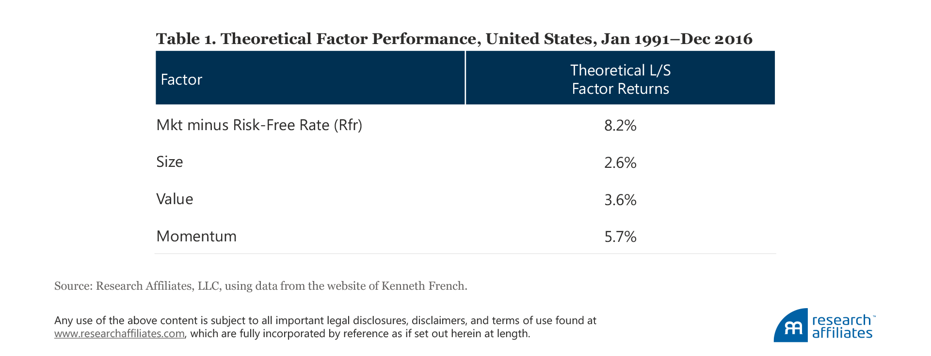
Factors are used to measure manager style, to disentangle style-based performance from skill-based performance, and to build and sell quantitative investment strategies. In addition to the capital asset pricing model, or CAPM, market factor, the value, size, and momentum factors are some of the more popular factors known to academics and practitioners since at least the early 1990s. Using the most common theoretical portfolio definitions, these four factors have shown quite impressive performance: the market, value, size, and momentum factors have delivered 8.2%, 2.6%, 3.6%, and 5.7% return a year, respectively, over the last 26 years! The low beta factor (also known as the betting-against-beta, or BAB, factor) discovered in the 1970s did not garner much popularity until recently, when it delivered an eye-catching 26-year return of 10.3%.4 Other factors that have become popular over the last decade—profitability, investment, and illiquidity—also showed fabulous historical returns of 3.9%, 3.2%, and 2.1% over the past quarter-century.
Such formidable numbers might suggest factor tilts are a ready path to higher returns as well as suggesting which factors are more likely to deliver outperformance going forward, and is the theory widely advanced as fact by a vocal quant community. This theory is also a product of data mining and selection bias. While theories can help advance our understanding of a subject, they are just idealized approximations of the real world built on a foundation of core—and often wrong—simplifying assumptions. No theory can fully capture how the real world works. Worse, the real world frequently presents us with objective facts and outcomes that contradict theoretical predictions.
Factor Returns: Theory Meets Practice
What if some factor returns earned by fund managers are far smaller than the historical theoretical factor returns imply, resulting in a return shortfall in investors’ real-world portfolios? In this case, the outputs of portfolio attributions based on theoretical portfolios will be inadequate and often misleading, and the investment process that takes theoretical factor performance for granted will favor factor tilts that fail to deliver in the real world. Ultimately, the knowledge that the returns achievable in practice differ starkly from the theoretical returns should urge investors to reconsider their factor allocation choices.
In practice, the long–short portfolios used to construct factor-return time series are not investable. The return histories for these paper portfolios ignore a startling array of costs associated with real-world implementation: trading costs, missed trades, illiquid stocks, commissions, management fees, borrowing costs for the short portfolio, and the use of stocks unavailable for shorting. To this list of return shortfall sources, we might add data mining and survivorship bias. By cherry-picking some factor histories, these factors can rise to the top of the popularity roster even when selected long after—and because of—the large returns they once earned.
We can measure, albeit with some imprecision, the return slippage or return shortfall. Factor attribution assumes that the factor return flows straight through to fund returns. Our goal is to find out, month by month, how much return a factor loading delivers to mutual fund results. We can “reverse engineer” factor returns from mutual fund returns using a two-stage regression procedure. The purpose of the first-stage regression is to help identify manager factor exposure (e.g., which fund is value and which fund is growth). Once we have the estimated factor exposure for all funds, the purpose of the second stage is to measure the performance difference between funds that is attributable to their different factor loadings (e.g., between value managers and growth managers) for each unit of factor exposure. 5
An example will help make our method easier to understand. For simplicity, suppose we have return data for two mutual funds (Fund A and Fund B) over a 12-month period. We first estimate the value factor loadings for each fund using the full 12-month sample of return data and conclude that Fund A is a value fund with a value beta of 0.6 and Fund B is a growth fund with a value beta of −0.3. Next, we calculate the monthly relative return of Fund A versus Fund B for each of the 12 months. Dividing each of the 12 monthly relative-return observations by the 0.9 value beta difference between the two funds, we can infer the return earned by each as a consequence of their different factor loadings.
For any two funds, the performance difference will be due to many contributing factors, not the least of which is idiosyncratic risk. Consequently, a performance difference will be a poor measure of the value factor return. But as the universe expands to include hundreds, and then thousands, of funds, we should be able to infer with some confidence the monthly returns attributable to each unit of value factor exposure.
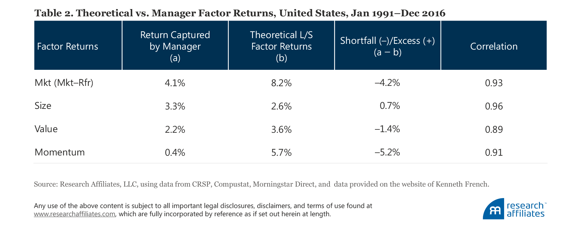
In a perfect world, the monthly factor returns derived from fund factor loadings, or the reverse-engineered factor returns, should very closely match the returns from the theoretical long–short portfolios used to create factors and factor-return time series. In fact, the returns derived from these two very different factor-return time series—one based on a long–short paper portfolio, and the other based on live fund returns—exhibit extremely high correlation (averaging over 90%). Month to month they track very closely. The mean returns, however, are shockingly different. Factor returns captured by mutual fund managers, especially for the factors with the largest historical long–short returns, tend to be starkly lower than their theoretical paper portfolio counterparts.
Our Data
Our analysis relies on data from Morningstar Direct Mutual Fund Database for the period January 1990–December 2016. The dataset reports historical monthly total returns for all mutual funds, including ones that were liquidated or merged, ensuring our mutual fund dataset is largely survivorship-bias free. The initial fund sample includes US open-end long-only active equity funds with at least two years of return history as of December 2016. We then limit the funds in our sample to A-share, no-load, and institutional share classes.6
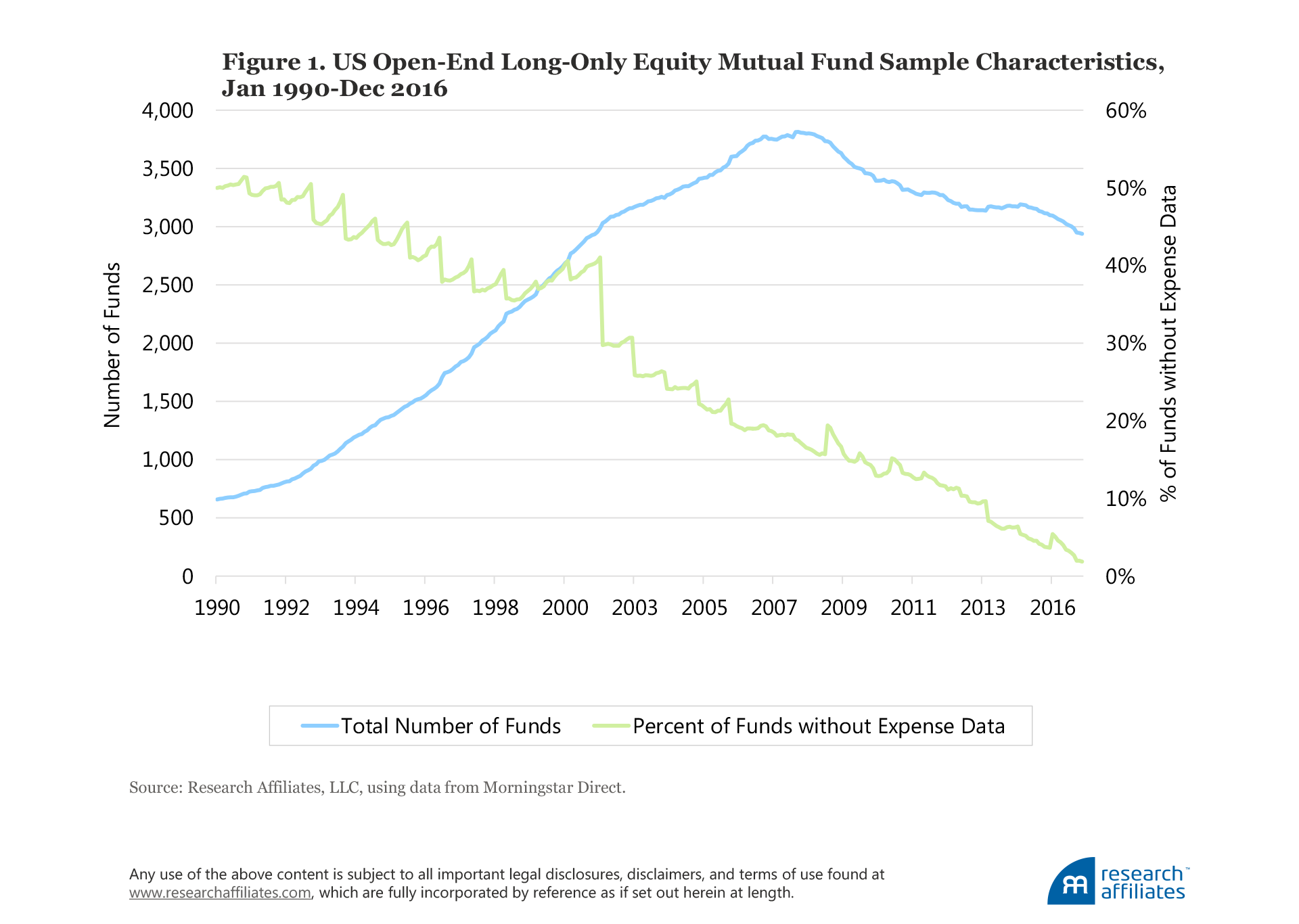
Our final US fund sample consists of 5,323 funds—a mixture of live funds and funds that no longer exist today. Figure 1 illustrates the evolution of the fund sample over time. Our sample size, the blue line, begins with 658 funds in 19907 (just over 392 unique funds not counting the different share classes) and gradually increases to a peak of 3,800 funds in 2008, before falling to about 3,000 funds in 2016.
The green line tracks the percentage of funds with reported returns, but without reported expense ratios. Information on fund expense ratios is not available for many funds, especially in the early part of the sample. Our main analyses use net-of-expense fund returns, which is how Morningstar Direct reports the data. For the subset of funds for which we do have expense data, we also conduct a robustness test showing results based on gross-of-expense fund returns.
Measuring Theoretical Factor Returns
For our analysis, we choose the four factors most widely used in manager performance evaluation: market, size, value, and momentum. We focus on these factors and ignore a myriad of the more recent, and sometimes exotic, factors in the “factor zoo.”8 We limit ourselves to these four, in part because the Morningstar Mutual Fund data we use starts in January 1990; if we were to include factors identified after the start of our data, we would be dealing with look-ahead bias.
Because these four factors were well known to investors prior to 1990 (or shortly thereafter), the theoretical factor returns, derived from long–short paper portfolios, and the investor’s realized factor returns, measured from actual fund performance, are both largely out of sample. The low beta factor was also known by the 1990s, but did not gain notable popularity until quite recently. Therefore, we exclude it from our main results, but explore it in detail in our robustness analysis later in the article.
The most common approach used by academics to measure factor returns follows the definition proposed by Fama and French (1993). The performance over the last quarter-century is impressive: all factors show positive performance.9 The market factor is the clear champion with an 8.2% annualized average return, followed by momentum at 5.7%. Value and size are well behind with annual returns of 3.6% and 2.6%, respectively. We report the theoretical factor performance in Table 1. The theoretical factor construction methodology is provided in Appendix A.
Following the Fama–French methodology, which is the most common theoretical factor definition, the market factor captures the monthly return difference between the market portfolio and US Treasury bills; the market portfolio weights all US large-cap stocks by market capitalization.10 The size factor captures the monthly return difference in the long–short portfolio between small-cap and large-cap stocks, controlling for value characteristics.
The value and momentum factors capture the performance difference in the respective factors’ long–short portfolios, which are constructed by selecting stocks based on the variable defining the factor, controlling for each firm’s market capitalization. Within both large-cap and small-cap groups (defined by median NYSE break points), we construct the long portfolio from the 30% of the market with the strongest value bias or momentum, and construct the short portfolio from the 30% of the market with the weakest value bias (strongest growth) or momentum. Both the long and short portfolios are cap-weighted.
In the Fama–French definition, the value and momentum factors equally blend the long–short factor portfolio constructed from large-cap companies and from small-cap companies. The intention of equally weighting the two portfolios is to control for the size factor while computing the other factor returns.11
These long–short paper portfolios are difficult, if not impossible, to replicate. Any implementation shortfall between the theoretical return of the paper portfolios and the factor returns realized by fund managers may be attributed to several possible sources:
- As already observed, paper portfolios ignore trading costs. This assumption is particularly important for factors with high turnover, such as the momentum and low beta factors.
- Paper portfolios typically extract more than half of the factor return from trading in stocks of small-cap companies, for whom trading costs are likely to be particularly high.
- In the real world, trades will be missed.
- Half of the return for most of these factors comes from the short side of the portfolio; in the real world, shorting may be expensive or impossible for some of the intended short sales.
- Paper portfolios ignore management fees, which are a direct and significant drag on investor performance.
- Theoretical factor returns assume that the historical prices for each individual stock, in each individual month, accurately reflect the prices at which an investor would be able to transact in the market place. Paper portfolios ignore stale prices and bid–ask spreads, which can be large for institutional-sized trades.
- Finally, the delisting bias documented by Shumway and Warther (1999) can further overstate performance for some factors. Shumway and Warther show that delisted stock returns recorded in the regular databases are much larger than what an investor would receive when transacting in the over-the-counter market, where these stocks are traded after being delisted.
These sources of implementation shortfall are unlikely to affect the long and short portfolios equally. For instance, many of these sources of implementation shortfall may exact a greater penalty on small-cap versus large-cap stocks (size factor), on value versus growth stocks (value factor), and on performance chasing versus contrarian investing (momentum factor).
Measuring Realized Fund Returns
We can measure the factor return slippage, albeit with some imprecision, by comparing the reverse-engineered factor returns we estimate from mutual fund returns to the conventionally constructed factor returns. Our reverse-engineering procedure starts with regressing mutual fund excess returns (the monthly fund return in excess of the risk-free rate) against factor returns to get each fund’s average factor loadings. For each mutual fund, we use the full-sample return data to estimate the factor loadings and ensure the accuracy and stability of the estimates.12 We then cross-sectionally regress fund returns for each month of history against the funds’ average factor loadings in order to extract the return that the funds realized, month by month, for each unit of factor exposure. We provide in Appendix B a detailed description of the two-stage regression-based methodology for the reverse-engineered manager factor premium.
With an example using mutual funds A, B, and C, we explain our regression process. In the first stage, we regress the full available history, over the roughly last quarter-century, of monthly mutual fund returns in excess of the risk-free rate for each of the three funds, separately, against the market, size, value, and momentum factor returns. The result is the respective beta of each of the factor exposures for each of the three funds over the periods the funds were live. The fund factor exposure estimates have look-ahead bias and ignore time-varying style shifts, as does historical factor-based return attribution, because we use fund full-sample returns for the estimation.
In the second-stage regression, for each month of data, we regress mutual fund returns (net of the risk-free rate) against the fund factor loadings estimated from the first-stage regression.13The second-stage regression coefficient for each of the factors gives us the monthly average return differences among mutual funds A, B, and C explained by the differences in the funds’ factor exposures. The monthly coefficient for each factor indicates the factor premium earned by the fund manager in that month, per unit of factor loading, which is the realized factor return we can compare with the theoretical paper portfolio factor return.
Our mutual fund return data sample includes a total of 324 months from January 1990 through December 2016. We conduct the second-stage regression analysis for every month, beginning January 1991 through December 2016. We ignore the first 12 months of data so our results will be directly comparable to the robustness tests we conduct later in the article.14 Therefore, for each factor, we have 312 monthly observations of estimated regression coefficients. Averaging these coefficients separately for each factor over time (i.e., across 312 monthly observations), we obtain the average factor premia captured by the fund managers.
We are following a standard empirical method known as a two-pass regression procedure for estimating factor premia that was introduced by Fama–MacBeth (1973). But instead of using theoretical portfolios with theoretical returns to estimate the factor premia, we use portfolios traded in the marketplace that are typical of the investor experience— we use net-of-expense mutual fund returns. Comparing the realized factor returns earned by fund managers to the theoretical factor returns from paper portfolios, we are able to measure the slippage associated with turning the theoretical factors into investment products accessible to investors.
A few possible criticisms of our approach, which we wish to acknowledge but do not address in this article, will be potentially addressed in our later research. The first possible criticism is that mutual funds may have time-varying factor loadings, whereas our method assumes static fund factor loadings. Also, our method may provide inaccurate return estimations (that is, the return captured by mutual fund managers) if managers frequently switch their investing styles.
A related potential issue with our methodology is that any factor loading estimates we obtain in the first stage are inherently noisy. The noisy measurement of loadings implies that the second-stage manager-captured factor premia estimates are downward biased relative to the “true” factor premia and may explain a portion of the slippage. At the same time, unless we assume that our factor sensitivities are significantly noisier for some factors than others, it would not explain why we observe materially different degrees of slippage for different factors.15
Another possible criticism is that if factor returns are driven by factor characteristics (such as direct observations of price-to-book ratio for value, past return for momentum, and market capitalization for size factors), our factor loadings, which are derived from regressions, may poorly capture the funds’ time-varying factor exposures.16 Perhaps, if the data were available, it would be better to measure the factor tilts directly using the same methods used to construct the paper factor portfolios. Again, we recognize this is a valid concern, which we will address in later work, observing that the same criticism could equally apply to factor-based historical return attribution.
Our Findings
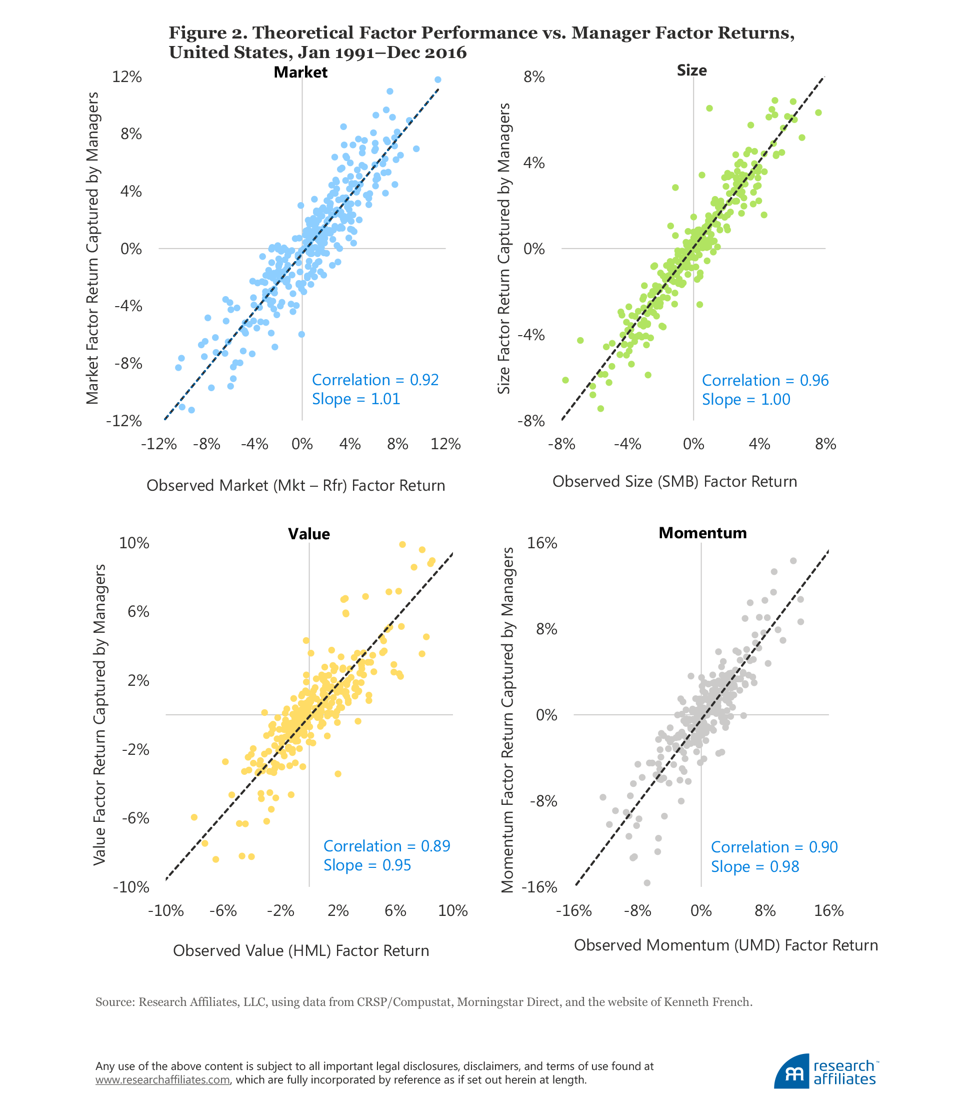
We now discuss our main results. Later in the article we provide a series of tests to study the robustness of our findings to model specification, share-class inclusion, and regional variations. How well do our reverse-engineered factors resemble the theoretical factor returns? Figure 2 displays the monthly returns of the theoretical portfolio plotted against the returns of our reverse-engineered factors; we also display the correlation and the slope coefficient between the two sets of return series. For all factors the correlation is in the range of 0.89 to 0.96 and the slope is in the range of 0.95 to 1.01. The average correlation is 0.92 and the average slope is 0.98, suggesting that the monthly behavior of the two sets of factor returns closely match each other.
Of course, the correlation between the two series only describes the co-movement between the two. Much more interesting is the average return the managers deliver for their exposure to the factors. In Table 2, for each of the four factors, we compare the average return captured by the managers and the average return delivered by the theoretical long–short factor portfolios. The average factor premia captured by the managers is significantly lower than that suggested by the theoretical returns for all factors with the exception of the size factor.
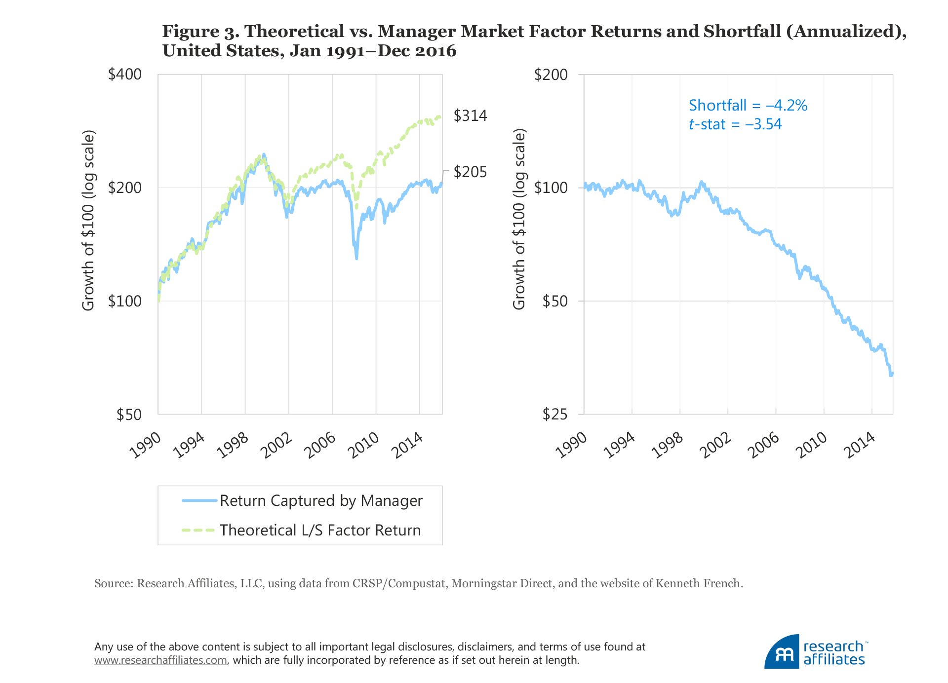
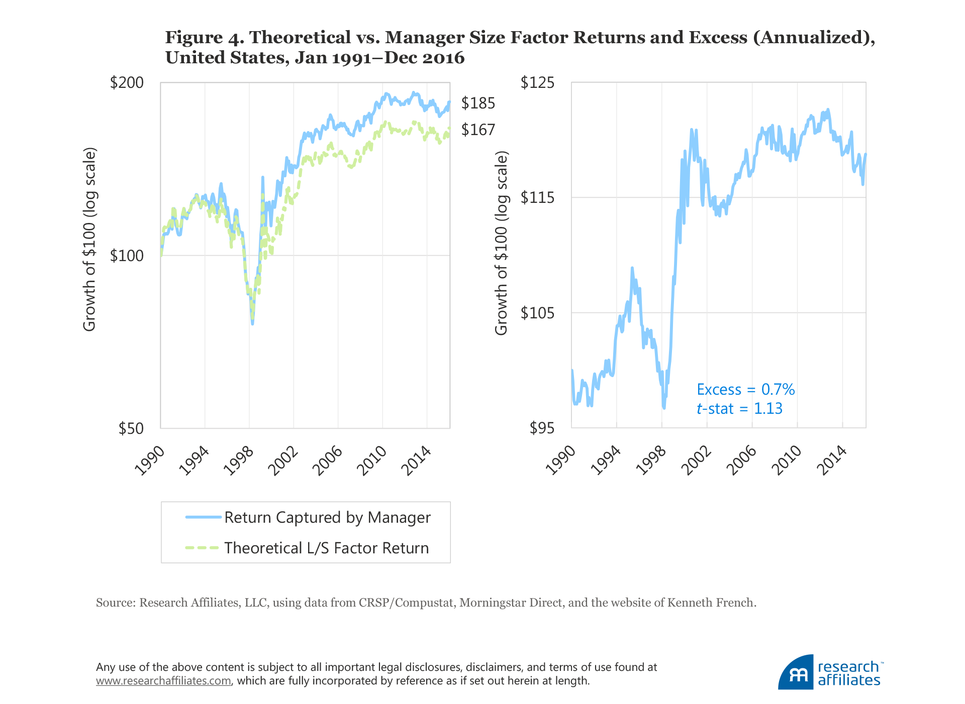
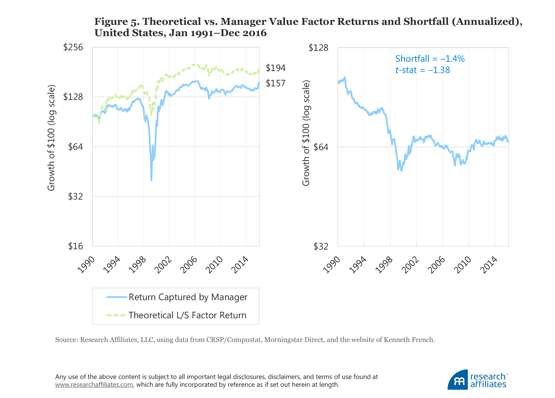
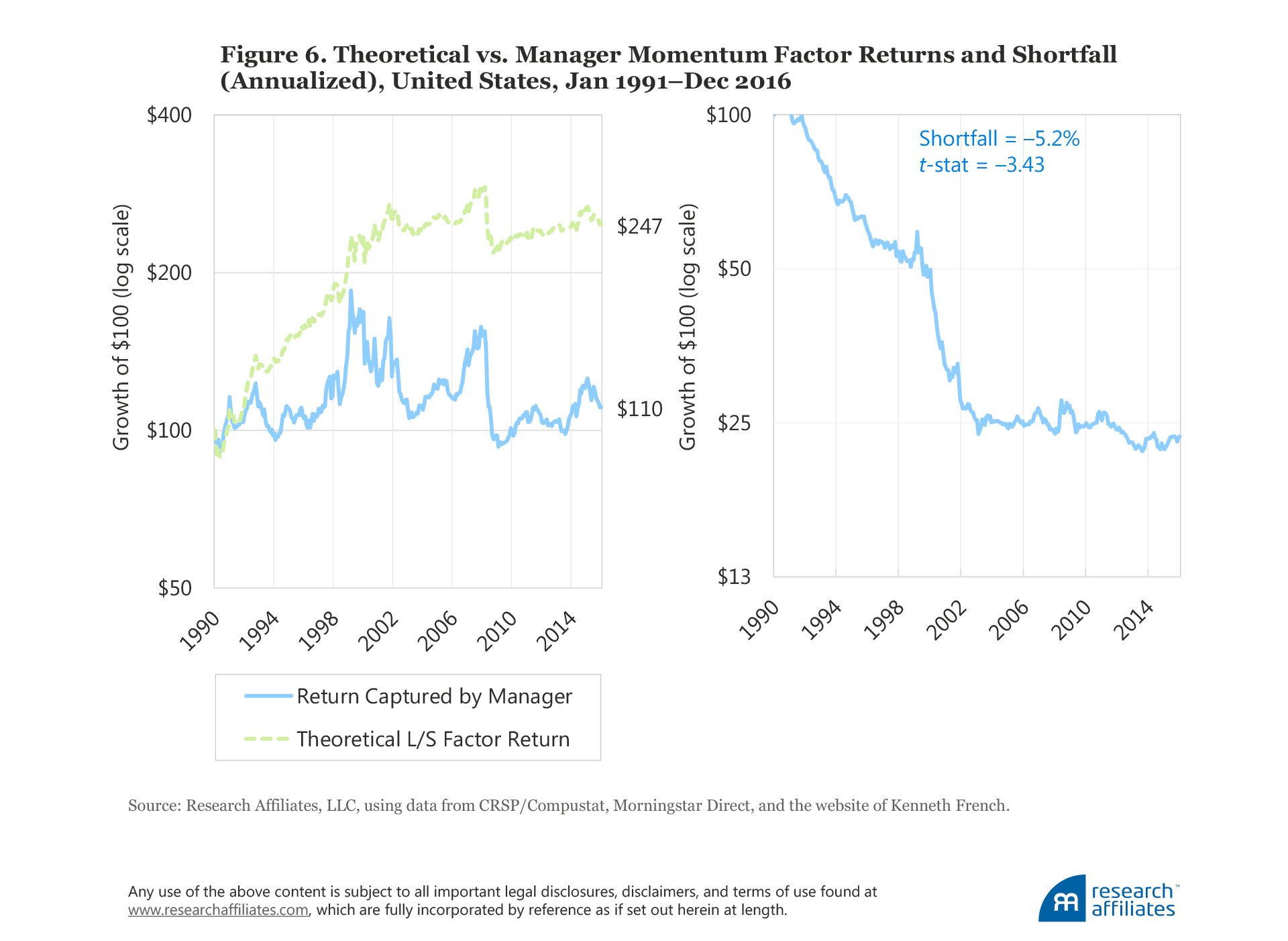
To show the evolution of factor performance—both theoretical and that delivered by managers, and the difference between the two—we produce two charts for each of the four factors. The first is a two-line chart in which the dashed line in the lighter shade represents the cumulative returns for theoretical long–short factor portfolios, and the solid line in the darker shade represents the cumulative returns of the factors realized by mutual fund managers; this chart provides a vivid demonstration of the fit of our reverse-engineered factor returns. The second is a one-line chart that plots the cumulative difference between the two factor returns—theoretical and realized by mutual fund managers.
Market Factor. Over the last 26 years, the factor return (net of transaction costs and other fees) earned by mutual fund managers by loading on market beta has fallen short of the observed equity market premium by 4.2 percentage points a year, as shown in Figure 3. The shortfall has a t-statistic of −3.54. In the first decade of our sample period, the reverse-engineered returns match the theoretical equity premium reasonably well, but the gap widens in the aftermath of the dot-com bubble, shrinking in the months before the global financial crisis, and widening again quite substantially in more recent years. For the market factor we have a reasonable explanation for the gap; for other factors the shortfall is harder to justify.
The market factor we use in our analysis reflects the return difference between stocks and cash. Over long periods of time, high beta stocks have been shown to underperform low beta stocks per unit of beta. Therefore, the gap we observe is not a surprise and is nothing more than the well-documented flat (or inverted in some studies) security market line,17 where differences in stock return performance are not explained by variation in market beta. Arguably, it might be considered surprising that the relationship is positive at all. One possible explanation for a positive realized market premium is the cash held by fund managers (and also, potentially, their use of leverage and derivatives), which introduces the conventional market-minus-cash beta sensitivity.
Size Factor. The theoretical and manager returns for the size factor demonstrate a near-perfect fit, with a correlation of 0.96, over our study period. The good fit is not a surprise. The turnover of the size factor (i.e., stocks migrating between the large-cap and small-cap categories) is one of the lowest among all conventional factors, making the funds’ replication of the factor quite easy. The extent of the good fit, however—that the size factor realized in mutual funds is stronger than the theoretical long–short size factor return—was a bit of a surprise.
Our findings, illustrated in Figure 4, suggest the cumulative return derived from mutual fund performance exceeds the theoretical long–short size factor returns by a small and not statistically significant margin (with a t-statistic of 1.13) of 0.7 percentage point a year. The surplus return may come from the ability to control transaction costs because turnover is low in small-cap portfolios. Further, we cannot rule out that some active small-cap managers may have better stock selection skills than their large-cap brethren.
Value Factor. The value factor premium is perhaps the most widely studied factor across world markets because value strategies are among the most widely embraced investment solutions in finance.18 Our research indicates, however, that most value strategies, when executed in the real world, leave much of the value effect on the table. This gap between theoretical and realized returns is rather persistent over our study period, with the exception of the first year. Over the last quarter-century, value managers captured only about 60% of the value premium indicated by the long–short value factor. Figure 5 shows that whereas a theoretical paper portfolio generated an annualized return of 3.6%, mutual fund managers were able to capture only 2.2% a year, an annualized slippage of 1.4 percentage points, with a t-statistic of −1.38.
Momentum Factor. The average annual return of the momentum factor based on long–short paper portfolios is 5.7% compared to the annualized factor return captured by momentum investors, which is close to zero, at 0.4% a year per unit of momentum loading. This shortfall, plotted in Figure 6, translates into an annualized slippage of 5.2 percentage points over the last quarter-century,19 with a t-statistic of −3.43! Most of the shortfall between the actual returns earned by fund managers and the theoretical paper portfolio happens by 2003, while essentially all of the alpha generated by the paper portfolio occurs prior to 2002.
Robustness Checks
We conduct several robustness checks to see if our results are unique to our initial project design. First, we remove look-ahead bias by recalibrating manager factor loadings to reflect fund returns preceding the month for which we are measuring realized factor returns. Second, we create an alternative long–short construction of the market factor return, comparing a low beta portfolio with a high beta portfolio. Third, we consider an array of newly popular factors including gross profitability (a popular quality measure), illiquidity, investment, and BAB. Fourth, recognizing that the performance slippage may be attributable to expense differences between momentum and anti-momentum funds, or between high beta and low beta funds, we test our results on the subset of funds for which gross-of-expense returns are available. Fifth, we test our results on an alternative fund sample where we keep only the oldest share class for funds that have more than one share class. Finally, we test our results on international funds against internationally based factor returns. All robustness checks produce results that support our core findings.
Factor sensitivity with no look-ahead calibration. The first step in our reverse-engineered factor return estimation is to measure the factor sensitivity of the funds. We use our full sample of fund return data to estimate the funds’ sensitivity to each of the four factors: market, size, value, and momentum. The factor loading estimates we obtain following this procedure are very accurate, but the procedure introduces look-ahead bias, which implies future knowledge of fund and factor performance.
Our first robustness check is to remove this look-ahead bias. Instead of using full-sample fund return data to estimate the factor loadings, we use only historical data. For the month whose factor return we are estimating, we use only the data prior to that month. For example, we use data from 1990 to 1999 to estimate the fund factor loadings, then regress January 2000 fund returns against the factor loadings to derive the realized factor returns for January 2000.
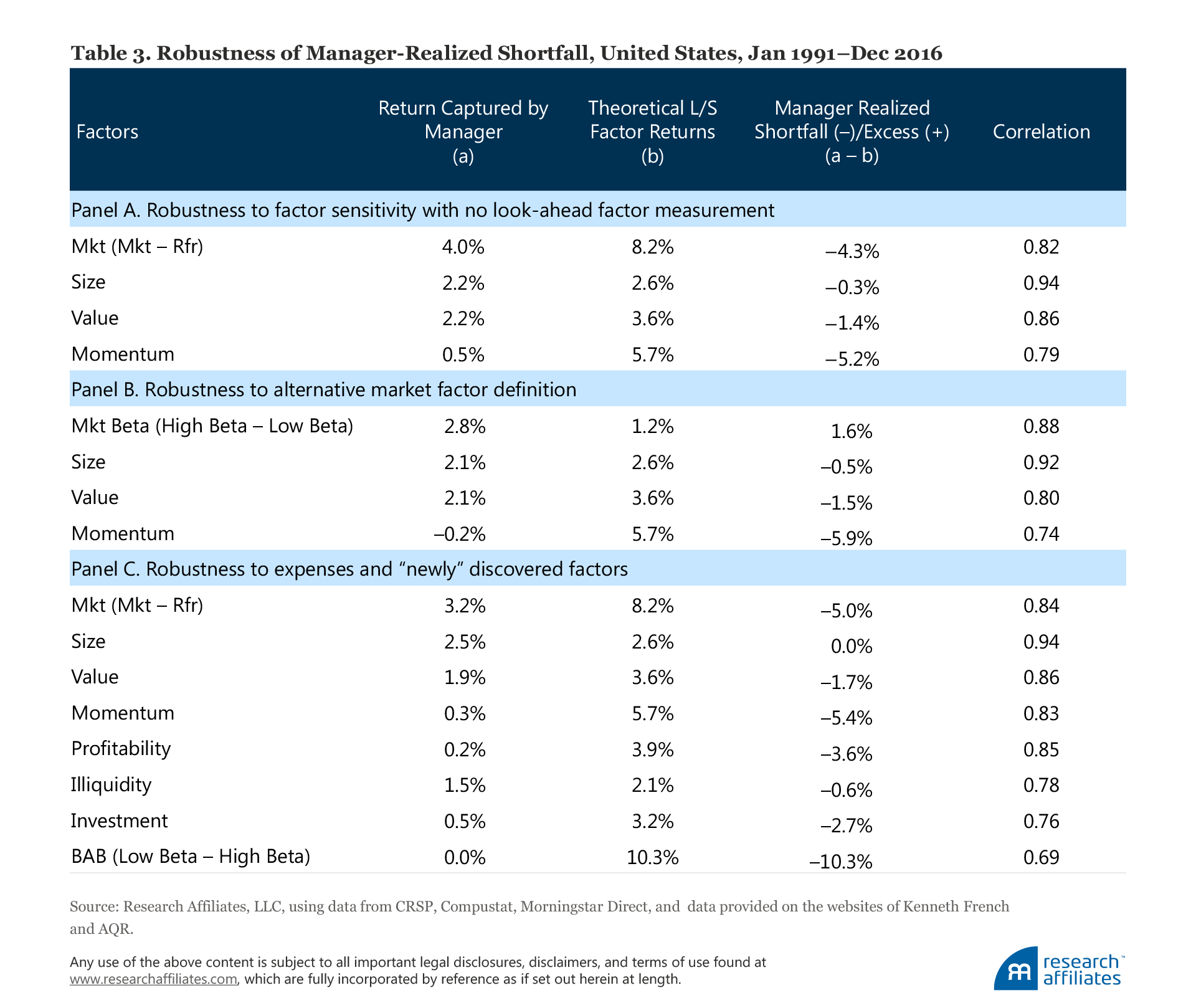
We report our results in Table 3, Panel A. The biggest difference is for the size factor; the excess of 0.7 percentage point we observe using the calibration with full-sample data turns into a shortfall of −0.3 percentage point when we eliminate look-ahead factor sensitivity measurement. Importantly, when we eliminate look-ahead fund factor sensitivities, the manager-realized shortfall/excess is largely the same; managers still capture close to the full size premium, about half the market and value premiums, and almost none of the momentum premium.
Alternative definition of market portfolio. In our earlier discussion about the potential explanation for the shortfall in the realized market factor return, we acknowledged the well-documented finding in the literature that high beta stocks do not outperform low beta stocks proportional to beta loading; a relationship empirically represented by a flat or inverted security market line. This potentially makes the market factor—stock return minus cash return—a poor benchmark for what we should expect as the return differences of funds with different market beta sensitivities.
To make a more apples-to-apples comparison, we respecify the market factor in a fashion very much like the approach taken in constructing the other factors, by constructing a long–short portfolio. We call this variant of the market factor the high-beta versus low-beta market factor. The long portfolio includes the 30% of the market with the lowest measured historical beta on a cap-weighted basis, and the short portfolio comprises the 30% of the market with the highest measured beta, cap-weighted.20 The leverage of the long–short portfolio is adjusted to keep the market beta of the portfolio equal to 1.0 in the full sample. Otherwise, we follow the no-look-ahead procedure for fund factor exposures described in our first robustness check. The results are displayed in Table 3, Panel B.
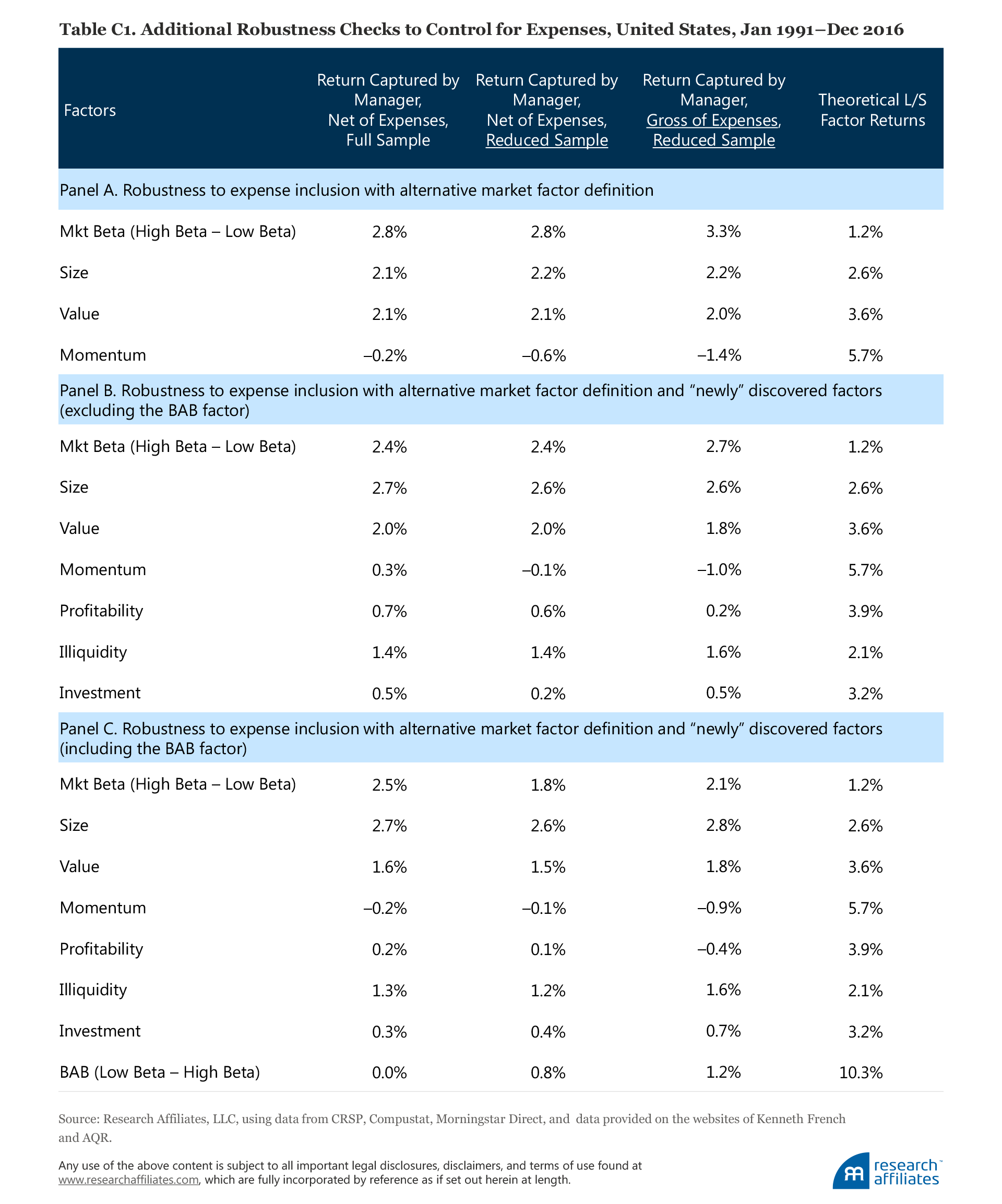
Using the alternative factor definition, the returns captured by managers through market exposure are reduced to 2.8% (a 1.2 percentage-point reduction compared to Panel A). The theoretical return for the market factor declines significantly more, from 8.2% in Panel A to 1.2% in Panel B. Because we do not change the other factor definitions, the theoretical factor returns for the other factors remain unchanged. The shortfall/excess of the factors is largely unchanged for size, value, and momentum. The difference in realized and theoretical returns changes significantly, however, for the market factor. The shortfall of −4.3 percentage points reported in Panel A is now an excess of 1.6 percentage points.
The change is driven mostly by the significant decline of 7.0 percentage points in the theoretical factor return, which drops from 8.2% to 1.2%. The other driver, which has a significantly smaller impact, is the decline of 1.2 percentage points, from 4.0% to 2.8%, in the return captured by the managers. These results are consistent with our earlier conjecture that the explanation for the deviation in the market factor return captured by fund managers compared to the theoretical factor return is driven by two forces: 1) a flat or inverted security market line, and 2) differences in the cash holdings between different managers, and potentially to a smaller degree by the use of leverage and derivatives. A high beta achieved by holding high beta stocks performs far worse than the market-minus-cash difference would predict. But a low beta achieved by holding cash performs far worse than the high-minus-low-beta factor would predict. So, these results are unsurprising.
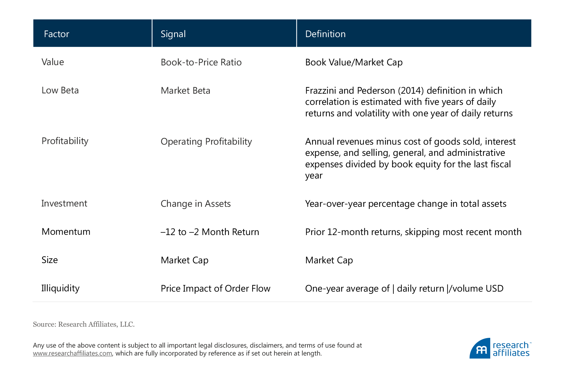
Including other factors. Until now, we have limited our analysis to the four most popular factors in the early 1990s. Considering today’s far-higher number of factors—316+ factors as of year-end 2012 (Harvey et al., 2012)—that have been “identified” by research published in top academic journals, unpublished manuscripts, second-tier academic journals, and practitioner journals, we ask if our results are robust to these other factors. But testing robustness to the inclusion of hundreds of factors is not practical. Instead, we choose to add to our analysis four additional factors that are very popular today: profitability, investment, illiquidity, and low beta, or BAB. We use the no-look-ahead calibration, which makes the Panel A results an appropriate comparison for the broader analysis. The results are presented in Table 3, Panel C.
For the four original factors in our analysis, we find that the manager-captured premia, and consequently the shortfalls, are largely unchanged; the biggest changes are the market factor premium, which declines by 0.8 percentage point from 4.0% to 3.2%, and the size factor premium for which the excess of 0.7 percentage point we observed earlier (Table 2) now disappears. The manager-captured factor premia for the four new factors we analyze are quite consistently close to zero, with the only exception being the illiquidity factor with a premium of 1.5%.
In the broader set of eight factors, over the last 26 years we find managers deliver a premium above 1% a year for only four: market, size, value, and illiquidity. All four of these factors are inherently uncomfortable to hold. Market risk is the biggest risk for most investors and is often correlated with the investor’s personal income because job losses and bear markets generally go hand in hand. The size factor may require investors to hold stocks they do not understand well and which have protracted periods of underperformance. The value factor is inherently uncomfortable to hold because value stocks are usually cheap for good reason, and a value strategy requires investors to sell recent winners and buy recent losers. The illiquidity factor’s level of discomfort for investors rests in not being able to sell investments without incurring large costs, typically at times when liquidity is most needed.21
Not all factors chase what is recently profitable and what is comfortable. Not all factors require frequent turnover to implement. Only those factors with low turnover, and which are uncomfortable to own, appear to be able to generate a return that can be captured by mutual fund managers.
Gross returns, before the total-expense ratio. All of our results presented thus far are based on net-of-expense returns. We now ask to what extent the shortfall in manager-realized factor returns can be attributed to the differences in expenses (primarily the management fee) between managers, especially between growth and value managers, between high-beta and low-beta managers, and between momentum and contrarian managers. We measure the sensitivity of our results to fund expenses by conducting two additional tests on the sample of funds for which we have expense information:
First, we analyze the subsample’s returns net of expenses to control for
1. the uneven distribution of expense information over the time sample, and
2. the potential for under-reporting due to self-reporting by fund managers, some of whom may choose not to report because of poor performance.
Second, we repeat the same exercise on a gross-of-expense basis.
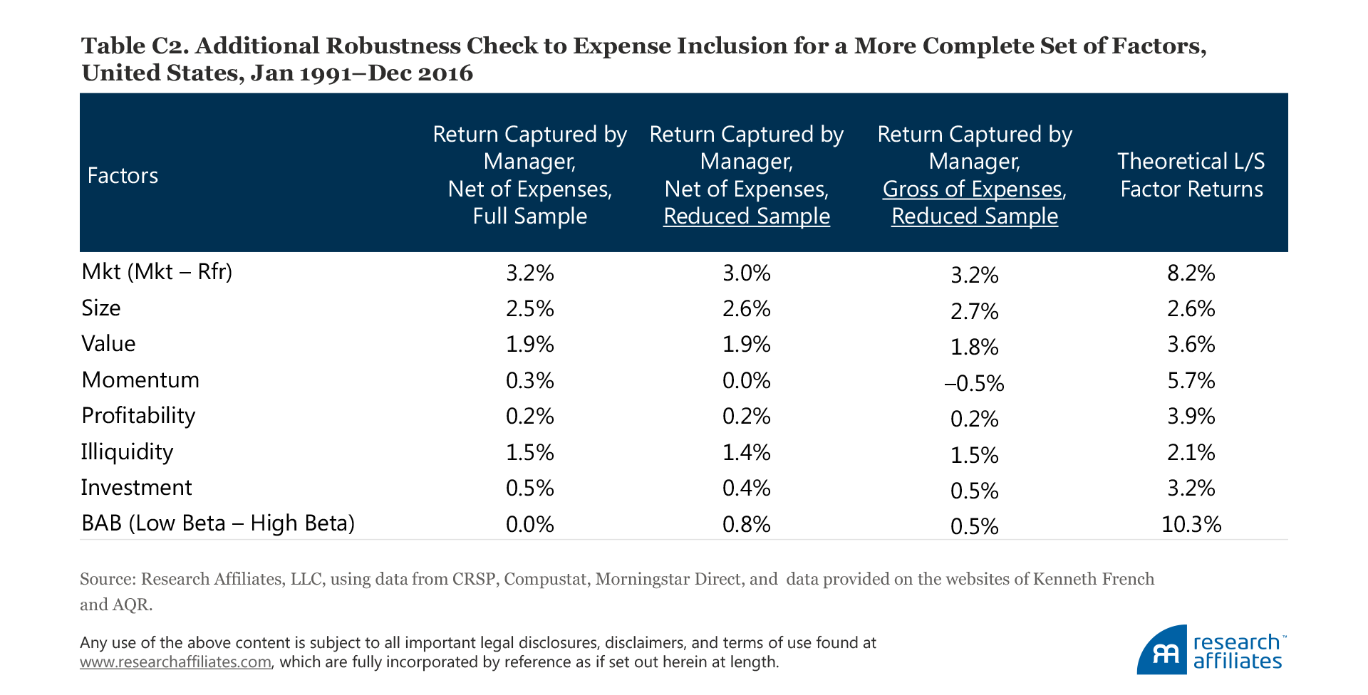
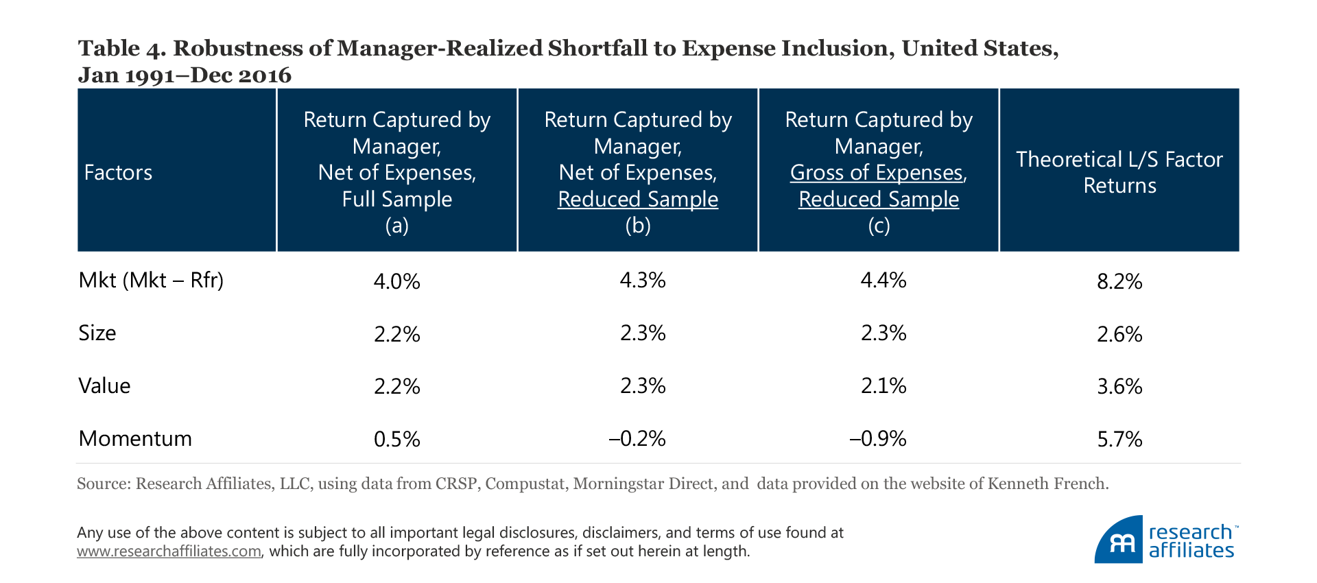
These test results are reported in Table 4. We do not have perfect coverage for the fund expense ratio, so we are only able to carry out our robustness tests on two different dimensions. The difference between column (a) and column (b) in Table 4 indicates the impact of the smaller sample size. The difference between column (b) and column (c) represents the impact due to expenses using the reduced sample of funds. In Table C2 of Appendix C we show additional tests for a more complete set of factors that are popular today; once again, controlling for expenses does not alter the results.
In a nutshell, the factor return shortfalls realized by fund managers are not driven by differences in expenses.
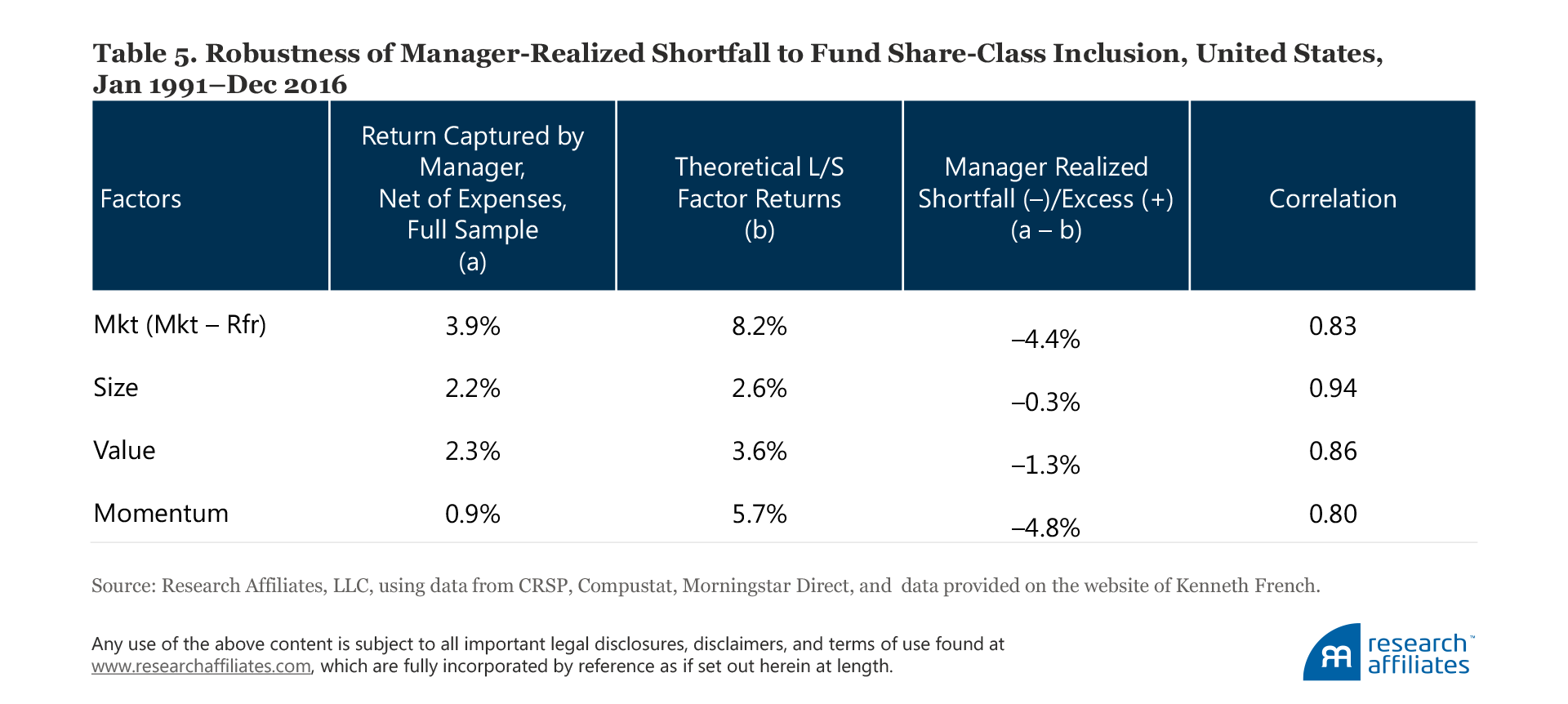
Alternative fund sample, keeping only the oldest share class for each fund. Some funds in our select mutual fund universe offer more than one share class; these classes have different shareholder rights and obligations, such as fee structures and load charges. All of our tests to this point include all three share classes (A-share, no-load, and institutional) if a fund in our sample offers all three. We treat each class as a separate fund. Mutual fund studies more commonly either consolidate multiple share classes by taking a weighted average based on total net assets or keep only the oldest share class of the fund. We now test the sensitivity of our results to our fund inclusion method by keeping only the oldest share class for those funds that offer more than one share class.
These results are reported in Table 5. The manager-realized factor shortfall/excess is largely unchanged. We conclude that our fund inclusion method does not bias our results.
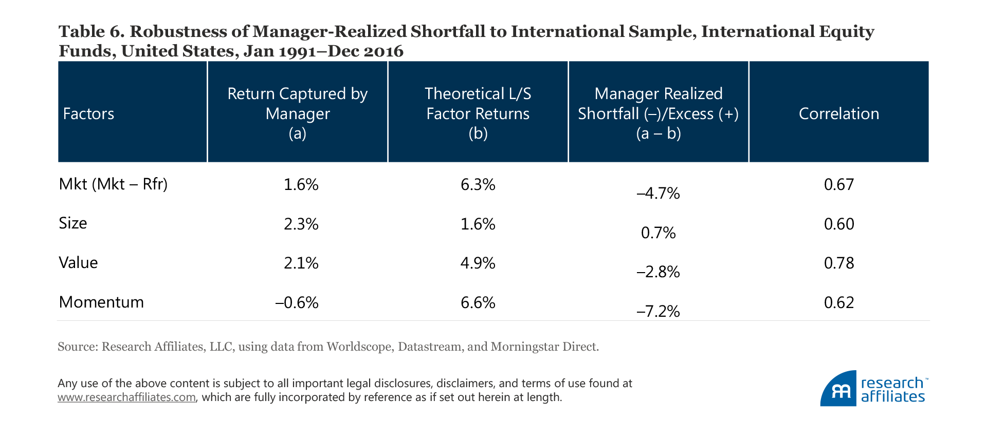
Manager-captured factor returns in international markets. Our findings so far reported are based on the US mutual fund data sample. International funds provide a good proving ground for an out-of-sample test. To form our international equity fund sample we select funds from the Morningstar Direct open-end long-only international equity universe that have at least two years of return history as of December 2016. We then limit our fund selection to A-share, no-load, and institutional share classes, following the same method we use to form our US fund sample. Our final international equity fund sample consists of 2,364 funds, a mixture of live funds and funds that no longer exist today.
We display in Table 6 the international results for the four most popular factors.22For the US fund sample, we are able to rely on the factor returns from the Kenneth French data library. The international fund sample, however, has some sizable emerging market positions. To ensure factor portfolio representativeness, we follow the standard Fama–French methodology in constructing the international (i.e., All World) long–short factor portfolios. Column (b) in Table 6 shows the historical premia for the factors, which are largely in line with the theoretical factor returns in the United States: market and momentum are the clear winners, followed by value and then by size. Returns captured by managers again fall significantly behind the theoretical returns. We observe the following:
- The market factor premium captured by managers, 1.6%, is significantly smaller than the theoretical market premium, producing a shortfall of −4.7 percentage points. This is quite consistent with earlier empirical work that finds a flat or sometimes inverted security market line, so our finding should not be a surprise.
- The size factor premium captured by managers, 2.3%, exceeds the theoretical factor premium by 0.7 percentage point. Just like in the US market, the international funds fully capture the size premium, and even capture a slight excess, which may be a sign of the stock-picking skill of small-cap managers.
- The value factor premium captured by managers, 2.1%, is the second largest after size, with a shortfall of −2.8 percentage points. Similar to our findings for US funds, the international funds capture slightly below half of the theoretical value premium.
- The momentum factor premium captured by fund managers is −0.6%, which results in a shortfall of −7.2 percentage points relative to the theoretical premium. Just like in the US market, the international funds do not capture the momentum premium.
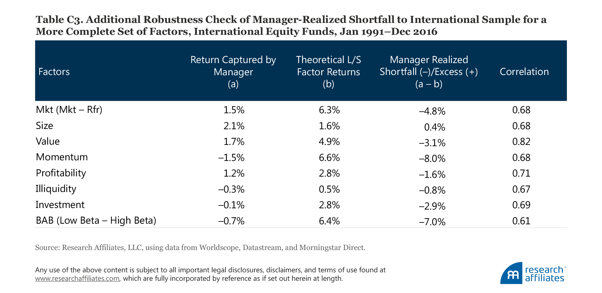
We also provide in Table C3 of Appendix C the results for a broader set of factors, those most popular today, for our international mutual fund sample. Controlling for other factors changes very little compared to the results for the main four factors. International fund managers, on average, capture a 1.2% a year profitability premium, representing a 1.6 percentage-point shortfall, much higher than in the US sample. Also different from the US results is that the illiquidity premium captured by managers is close to zero, −0.3% a year, in the international market, whereas it is slightly positive at 1.5% in the US market.
The international findings support our US findings: managers fully capture the size premium, capture less than half of the value and market premiums, and capture essentially nothing of the momentum premium, although they do capture the ups and downs as momentum wins and loses.
The Source of the Slippage
Our results show high slippage for the market factor. This is no surprise. A flat security market line is well documented: differences in stock return performance are not explained by variation in market beta. Indeed, the only reason we likely show a positive realized factor return for the market factor is managers’ use of cash and derivatives, which have the conventional market-minus-cash beta sensitivity. For the long–short factors, our results show little-to-no slippage for size, moderate slippage for value, and a very high slippage for the momentum factor.
Theoretical portfolios ignore the costs to trading and shorting and rely heavily on small and illiquid stocks, which are associated with higher costs to trade. They ignore management fees and other costs related to implementation, causing a shortfall in the realized factor return versus the theoretical return.
How big are the transaction costs associated with implementation of different factors? Several studies, including Novy-Marx and Velikov (2015) and Beck et al. (2016), show that low-turnover strategies, such as value and size, incur small to moderate trading costs. The higher-turnover strategies, such as momentum (and to a lesser extent low volatility, or BAB), have trading costs that may be large enough to wipe out the premium completely if enough money is following the strategy. This order matches the slippage we observe in our study and suggests that transaction costs likely play a major, even dominant, role as the source of slippage between theoretical and realized factor returns.
Another possible source of slippage could be manager skill in choosing the negativefactor exposure. For example, if growth fund managers have strong stock-selection or timing skills, the difference in performance between value and growth managers will appear as an erosion in the realized value premium, when computed using our method, versus the theoretical value premium. We will explore the possible drivers of factor return slippage later in our series of articles. Meanwhile, caveat emptor!
Are Investors Believing in Impossible Things?
Factor investing is gaining popularity in the investment community. To some degree, the practitioners are catching up with the academic research—this is a good thing because investors’ toolkits are being enriched. Yet, we must wonder, if 10,000 quants are all pursuing the same factor tilts, how likely are they to add value? The use of academic tools, without proper understanding of hidden costs or of the ways to mitigate implementation shortfall, can lead to tears. We would argue this is already happening.
Whereas theoretical factor returns offer a rich array of tools to use in return attribution and for portfolio construction, these long–short paper portfolios are taking aggressive positions among small and potentially very illiquid groups of stocks. If investors assume that the paper-portfolio returns from these factors can be earned in the real world, they may be in for a big surprise. The paper portfolios ignore trading costs and management fees, and assume that the data at which prices are recorded in the theoretical return databases accurately reflect the trading opportunities. These theoretical factors are selected today with the blessings of hindsight, data mining, and selection bias. Of course their historical results look brilliant!
We find that fund managers experience significant shortfalls in their ability to capture factor returns compared to theoretical paper portfolios. In particular, the shortfall is quite strong for the market and value factors, where the return delivered to the end-investor is halved or worse. For the momentum factor the end-investor seems to have enjoyed no benefit whatsoever from fund momentum loadings nor any penalty for funds that have an anti-momentum bias. We suspect the lion’s share of the shortfall is due to trading costs, a topic we may explore in a future article. Factor returns are inherently uncertain, whereas some drivers of slippage, such as costs or returns, which are not captured by the short side of the paper portfolio are a lot more predictable. If these predictable factors are responsible for the slippage, we are likely to see a similar magnitude of slippage in the future.
Endnotes
1. In 2016 we published three articles on the time variation of factor and smart beta strategy returns: “How Can ‘Smart Beta’ Go Horribly Wrong?”, “To Win with ‘Smart Beta’ Ask If the Price Is Right,” and “Timing ‘Smart Beta’ Strategies? Of Course! Buy Low, Sell High!”
2. The fact that factor tilts and smart beta strategies are expensive has two uncomfortable implications. First, the past success—often only as simulated past performance—is partly a consequence of revaluation alpha from these strategies enjoying a tailwind as they became more expensive. As investors, we extrapolate that part of the historical alpha at our peril. Second, any mean reversion toward historical norms for relative valuation could turn positive historical alpha into negative future alpha.
3. We were excoriated by some critics for suggesting that some so-called smart beta strategies could “go horribly wrong” and for suggesting the risk of a “smart beta crash” in some strategies, analogous to the quant crash of August 2007. In the second half of 2016, after we published “To Win with ‘Smart Beta’ Ask If the Price Is Right,” low vol lost money in a bull market. At this writing, in the eight months since June 2016, low-volatility strategies have lagged value strategies by over 1,000 basis points in the US, international, and emerging markets. Quality and momentum strategies were hit about half as hard relative to value. The two smart beta strategies we identified as cheap (value and size) have fared well, and the three we identified as rich (profitability, momentum, and low vol) all fared poorly. Did some smart beta strategies “go horribly wrong”? Absolutely.
4. The low beta effect was documented by academia in the 1970s, however, the BAB factor research was only published in 2014 and became popular in recent years.
5. This method introduced by Fama and MacBeth (1973) is frequently used in academic publications.
6. The Morningstar Direct Mutual Fund Database includes liquidated or merged funds. We focus on institutional, no-load, and A-share classes because they are the most relevant to retail and institutional investors. These three classes differ in fee structures and represent investment returns to different types of investors. Inclusion of all three share classes enriches the sample. Also, the inclusion of multiple share classes should not bias the slope of the second-stage regression coefficients (the methodology is described in the Appendix) nor therefore our conclusions based on our findings.
7. Before 1990, given the small number of unique funds, our test estimating the multifactor premia may run into identification problems.
8. John Cochrane coined this marvelous expression. Harvey et al. (2015) show that over 316 factors were “discovered” and published in the academic research by year-end 2012, with over 90% of that research published since 2000. In conversations with Cam Harvey, he suggested that all 316 exhibited positive alpha, almost all showed statistical significance net of the size and value factors, and none of the researchers—zero—had tested whether their strategy had enjoyed a tailwind of rising relative valuations, which may have driven part or all of the factor’s historical efficacy.
9. Of course, if they did not have positive performance, they would not have become popular!
10. The US large-cap equity universe consists of stocks whose market capitalizations are greater than the median market capitalization on the NYSE.
11. The outcome, however, may be quite different from the intent. For many factors, the returns within the universe of large and small stocks are materially different. Typically, the factors constructed within the universe of small stocks exhibit significantly higher risk and frequently higher premia than the results for the large-stock universe. Measured by market capitalization, the small-cap universe only represents about 10–20% of the entire equity market. Equally weighting the large-cap and small-cap portfolios essentially increases the impact of the small-cap market segment to 50%, which increases performance of the theoretical portfolio and potentially overstates the achievable factor premia. Nevertheless, because the goal of this article is to compare the theoretical versus the realized factor premia, we follow the most commonly accepted definitions of the factor portfolios.
12. In a later section of the article where we test the robustness of our results, we use an alternative ex ante estimation with largely unchanged conclusions. Although the original Fama–Macbeth (1993) methodology uses only ex ante data in measuring portfolio factor loadings, Fama and French (1992) tested and concluded that using full-sample data for factor loading estimation does not lead to material differences in factor premia estimation.
13. Each fund’s factor loadings used in the second stage of the regression are identical throughout all months because the loadings are calculated using the fund’s full-sample returns.
14. In our robustness tests, because we use only ex ante information in our factor beta estimations in the first-stage regression, and we start the first set of factor beta estimations only after having at least 12 months of return data, January 1991 is the first month (using all available data up to December 31. 1990) for which we have the first set of factor beta estimations. Therefore our ex ante test results start from January 1991.
15. Differences in ex post correlations of implied manager premia and paper factor portfolio premia do not reveal much about the slippage relationship.
16. A long-lasting debate in the academic literature is whether risk exposures or stock characteristics is the better driver of expected returns. Fama and French (1993) argue that returns are driven by risk exposures, while Lakonishok, Shleifer, and Vishny (1994) argue that mispricing and stock characteristics may be the stronger driver. Daniel and Titman (1997) conduct a test comparing the two hypotheses and conclude that stock characteristics may be a better driver. Evidence on both sides of the debate comes from Berk (2000) and Davis, Fama, and French (2000), who argue that risk exposures are more important, and Daniel, Titman, and Wei (2001) and Chaves et al. (2013), who argue stock characteristics are more important.
17. In the early 1970s, researchers such as Haugen and Heins (1975) and Black, Jensen, and Scholes (1972) found empirical evidence that variation in market beta risk is not matched with compensation for risk; this is known as a flat or sometimes inverted security market line.
18. The value effect was first documented by Basu (1977). The two most accepted explanations for the value effect are risk based, as proposed by Fama and French (1992), and behavioral, as proposed by Lakonishok, Shleifer, and Vishny (1994).
19. The apparent 0.1 percentage-point difference is due to rounding.
20. We follow Frazzini and Pederson (2014) to calculate stock market beta, in which correlation is estimated with five years of daily returns, and volatility with one year of daily returns.
21. We have often said that finance theory got off on the wrong track well over a half-century ago with the notion of a risk premium. Had it been called a “fear premium” most of the anomalies of modern finance would have been fully expected and the merging of behavioral and neoclassical finance would have been a fait accompli many years ago.
22. Our results for factor sensitivity of the funds is measured with no look-ahead bias.
References
Arnott, Robert, Noah Beck, and Vitali Kalesnik. 2016a. “To Win with ‘Smart Beta’ Ask If the Price Is Right.” Research Affiliates (June).
———. 2016b. “Timing ‘Smart Beta’ Strategies? Of Course! Buy Low, Sell High!” Research Affiliates (September).
Arnott, Robert, Noah Beck, Vitali Kalesnik, and John West. 2016. “How Can ‘Smart Beta’ Go Horribly Wrong?” Research Affiliates (February).
Basu, Sanjoy. 1977. “Investment Performance of Common Stocks in Relation to Their Price-Earnings Ratios: A Test of the Efficient Market Hypothesis.” Journal of Finance,vol. 32, no. 3 (June):663–682.
Berk, Jonathan B. 2000. “Sorting Out Sorts.” Journal of Finance, vol. 55, no. 1 (February):407–427.
Black, Fischer, Michael C. Jensen, and Myron Scholes. “The Capital Asset Pricing Model: Some Empirical Tests.” In Studies in the Theory of Capital Markets, edited by M. C. Jensen. New York: Praeger, 1972.
Chaves, Denis, Jason Hsu, Vitali Kalesnik, and Yoseop Shim. 2013. “What Drives the Value Premium? Risk versus Mispricing: Evidence from International Markets.” Journal of Investment Management, vol. 11, no. 4 (Fourth Quarter):1–18.
Daniel, Kent, and Sheridan Titman. 1997. “Evidence on the Characteristics of Cross-Sectional Variation in Stock Returns.” Journal of Finance, vol. 52, no. 1 (March):1–33.
Daniel, Kent, Sheridan Titman, and John Wei. 2001. “Explaining the Cross-Section of Stock Returns in Japan: Factors or Characteristics?” Journal of Finance, vol. 56, no. 2 (April):743–766.
Davis, James, Eugene Fama, and Kenneth French. 2000. “Characteristics, Covariances, and Average Returns: 1929 to 1997.” Journal of Finance, vol. 55, no. 1 (February):389–406.
Fama, Eugene, and Kenneth French. 1992. “The Cross-Section of Expected Stock Returns.” Journal of Finance, vol. 47, no. 2 (June):427–465.
———. 1993. “Common Risk Factors in the Returns on Stocks and Bonds.” Journal of Financial Economics, vol. 33, no. 1 (February):3–56.
———. 2012. “Size, Value, and Momentum in International Stock Returns.” Journal of Financial Economics, vol. 105, no. 3 (September):457-472.
———. 2015. “A Five-Factor Asset Pricing Model.” Journal of Financial Economics, vol. 116, no. 1 (April): 1-22.
Fama, Eugene, and James MacBeth. 1973. “Risk, Return, and Equilibrium: Empirical Tests.” Journal of Political Economy, vol. 81, no. 3 (May/June):607–636.
Frazzini, Andrea, and Lasse Heje Pedersen. 2014. “Betting Against Beta.” Journal of Financial Economics, vol. 111, no. 1 (January):1-25.
Harvey, Campbell, Yan Liu, and Heqing Zhu. 2015. “...and the Cross-Section of Expected Returns.” Review of Financial Studies, vol. 29, no. 1 (January):5–68.
Haugen, Robert A., and A. James Heins. 1975. “Risk and the Rate of Return on Financial Assets: Some Old Wine in New Bottles.” Journal of Financial and Quantitative Analysis, vol. 10, no. 5 (December):775–784.
Hsu, Jason, Vitali Kalesnik, Noah Beck, and Helge Kostka. 2016. “Will Your Factor Deliver? An Examination of Factor Robustness and Implementation Costs.” Financial Analysts Journal, vol. 72, no. 5 (September/October):58–82.
Lakonishok, Josef, Andrei Shleifer, and Robert Vishny. 1994. “Contrarian Investment, Extrapolation, and Risk.” Journal of Finance, vol. 49, no. 5 (December):1541–1578.
Novy-Marx, Robert, and Mihail Velikov. 2015. “A Taxonomy of Anomalies and Their Trading Costs.” Federal Reserve Bank of Richmond working paper (August).
Shumway, Tyler, and Vincent Warther. 1999. “The Delisting Bias in CRSP’s Nasdaq Data and Its Implications for the Size Effect.” Journal of Finance, vol. 54, no. 6 (December):2361–2379.
Appendix A. Theoretical Factor Construction Methodologies
For US factor portfolios, we use the published factor returns available through the Kenneth French Data Library for the following factors: market, size, value, momentum, profitability, and investment. For the US low beta factor, we use the published returns from the AQR website.
For international factor portfolios, we use the universe of stocks from the Worldscope/Datastream database. We define the international large-cap equity universe as stocks with market capitalization in the top 90% by cumulative market-cap within their region, where regions are defined as Japan, United Kingdom, and Europe ex UK. The small-cap universe is defined as the bottom 10% by cumulative market-cap.
We divide each universe by the various factor signals to construct desired-characteristic (the long side) and undesired-characteristic (the short side) portfolios. We follow Fama and French (1993, 2012, 2015) in constructing value, size, profitability, investment, and momentum factor portfolios in both large- and small-cap universes. For example, to simulate the large-cap value factor in the United States, we construct the value portfolio from large-cap stocks above the 70th NYSE percentile by book-to-market ratio (desired characteristic), and we construct the growth portfolio from large-cap stocks below the 30th NYSE percentile (undesired characteristic). To simulate the small-value factor in the international markets, we construct the value portfolio from small-cap stocks above the 70th percentile in their respective region (Japan, United Kingdom, and Europe ex UK) by book-to-market ratio, and the growth portfolio from small-cap stocks below the 30th percentile in their respective region.
Each long-side or short-side portfolio is defined as the equal-weighted average of large- and small-cap portfolios. These portfolios are weighted by market capitalization and rebalanced annually each July, with the exception of momentum, which is rebalanced monthly. The long- and short-side portfolios are then used to form a long–short factor portfolio without leverage. For example, the value factor is the average return on small-value and large-value portfolios minus the average return on small-growth and large-growth portfolios:

We follow Frazzini and Pedersen (2014) in constructing the low beta factor. We use the median value as the breakpoint instead of the 70th and 30th percentiles. The high-beta and low-beta portfolios are weighted by the difference between beta ranks and average rank, and rebalanced monthly. The long–short portfolio is a self-financing zero-beta portfolio with leverage:

Appendix B. Two-Stage Regression-Based Methodology for Reverse-Engineered Manager Factor Premium
For n fund returns and m factors, the first stage obtains the factor exposure βs by calculating n regressions on each of m factors, as follows:

Where Ri,t is the return of fund i (n total) at time t; Fj,t is the factor j (m total) at time t; βi,Fm are the factor exposures that describe how returns are exposed to the factors; and t goes from 1 through T. Note that each regression uses the same factors, F, because the purpose is to determine the exposures of each fund’s return to a given set of factors.
The second stage is to compute T cross-sectional regressions of the returns on the m estimates of the βs (we can call them B̂) calculated in the first stage. Each regression uses the same βs from the same step:

where γ are regression coefficients that are later used to calculate the risk premium for each factor. In each regression, i goes from 1 through n (n funds).
These two steps are followed by m series of γ coefficients, one for every factor, each having length T. The risk premium γm for factor Fm is the simple average of γm over time.
Appendix C. Additional Robustness Checks
