
Timing “Smart Beta” Strategies? Of Course! Buy Low, Sell High!
A contrarian timing approach—emphasizing factors or strategies trading cheap relative to their own historical norms, and deemphasizing the more expensive factors or strategies—can improve performance, but should be used in moderation to avoid increasing portfolio risk from a loss of diversification.
Contrarian timing is a form of value investing, but is not the same as doubling down on value risk. Relative valuation may support investing in the value factor when value is cheaply priced, and conversely, may indicate avoiding the value factor when it is expensive.
Most investors already practice a form of market “timing” by performance chasing, which can erode the benefits of factor investing even when diversifying across factors having recent strong results.
Valuations matter. Smart beta strategies and factors trading at a discount to their historical norms are poised to deliver positive performance in the crowded smart beta investing space.
This is the third of a series on the future of smart beta.
In the first article—“How Can ‘Smart Beta’ Go Horribly Wrong?”—we show that performance chasing can be as dangerous in smart beta as it is in stock selection, fund selection, or asset allocation. We differentiate between “revaluation alpha” and “structural alpha.” The former is the part of the past return that came from rising valuations.1 Revaluation alpha is nonrecurring, and is at least as likely to reverse as to persist. Rising valuations create an illusion of alpha and encourage performance chasing.
Structural alpha is the part of the past return that was delivered net of any impact from rising valuations. Why do we emphasize rising valuations? Because factors and strategies with tumbling valuations are rarely noticed in the data mining so pervasive throughout the finance community.2 For some factors, such as low beta, we show that most or all past performance was revaluation alpha, which could easily reverse from current valuation levels. For smart beta strategies, the picture is a bit better: most established products have respectable structural alpha.3
In the second article, “To Win with ‘Smart Beta’ Ask If the Price Is Right,” we show that valuations are predictive of future returns. We demonstrate that this result is robust across time, in international and emerging markets, and holds for various metrics used to measure valuations. We also point out that—for the moment, at least—many so-called smart beta strategies are trading in the top quartile, and even top decile, of historical valuations. We caution those who believe past is prologue and are tempted to extrapolate past “alpha” into expected future returns without regard to current valuation levels.
In this article we explore whether active timing of smart beta strategies and/or factor tilts can benefit investors. We find that performance can easily be improved by emphasizing the factors or strategies that are trading cheap relative to their historical norms and by deemphasizing the more expensive factors or strategies. We also observe that aggressive bets (favoring only the cheapest factor or smart beta strategy) can severely erode Sharpe ratios, so that gentle or moderate tilts toward that factor or strategy would seem to be a sensible compromise. Finally, we note that both factor and smart beta strategies have typically been identified and accepted as potentially alpha generating by the finance and investing communities after a period of impressive success—indeed, many of our own tests include a span that predates their discovery. We show that out-of-sample tests, after a strategy or factor has been discovered, are often far less impressive.
We Are All Market (and Factor) Timers!
How many times have we been drawn to a strategy, factor tilt, fund or ETF, asset class, or individual stock based on its past performance, goaded by a fear we’re missing out? How often are we repelled when a strategy, factor, fund, or manager has been persistently disappointing, driven by a concern that past is prologue? In seeking new sources of diversification, how often do we ask if the winners are newly expensive, poised to disappoint, or if the losing investments we may be ready to drop are newly cheap, poised to provide wonderful results? How often do we even consider selecting a poorly performing investment or strategy, thinking it may now be cheap? In each of these examples, we’re not only market timing, we’re performance chasing.
We’re all market timers, even in the halls of academe. Value investing goes back centuries, but the value factor, per se, wasn’t “discovered” in academic literature until 1977.4 In 1977, the Fama–French value portfolio (the 30% of the market with the highest book-to-price ratio) was priced more richly relative to the growth portfolio (the 30% with the lowest book-to-price ratio) than ever before or since, in data back to 1926. Similarly, the size effect was first published in the academic literature in 1981, near the end of its impressive 1975–mid-1983 run, and just ahead of a disastrous 15 years through 1999, during which the cumulative wealth of the Russell 2000 investor fell by more than half relative to the Russell 1000 investor.
Our experience from interacting with clients, investors, and market pundits suggests that many—including sophisticated large institutional investors—are already timing factors and smart beta strategies.5 Unfortunately, many are doing so in a self-destructive way by trimming reliance on newly cheap factors and strategies, while increasing allocations to newly expensive factors and strategies, activities detrimental to both Sharpe ratios and returns. Many investors have recently been scrambling to diversify their exposure to value. Is that not market timing and performance chasing? Of course it is!
When evaluating managers, mutual funds, and strategies, common practice is to look at both recent and long-term performance. Disappointing recent fund performance can be seen as a signal that the manager has “lost it,” perhaps by exhausting a source of alpha. Alternatively, it may signal that the manager did not have the skill to outperform in the first place. The possibility that the manager’s strategy is newly cheap (and therefore attractive) is rarely considered. A three- or five-year span, and often even a shorter spell, of underperformance—in extreme cases, just a few quarters—can suffice to get a manager fired; consequently, a subsequent reversal of shortfall would never be observed because the manager no longer manages the divested assets. To replace the underperforming managers, investors usually reallocate the divested funds to managers who have recently delivered wonderful performance.
Today in smart beta land we notice similar behavior. If a factor underperforms for multiple years (e.g., value’s recent nine-year span in the dog house!), investors question if the factor (or strategy) still works. Losing confidence in a particular strategy or factor, they may abandon it, trim it, or seek complementary strategies to diversify their risk. What strategies draw their attention? Generally only strategies or factors with superior recent performance.
Relative Valuation and Timing: How Well Does It Work?
Our first two articles explore the link between a strategy’s valuation and its performance. Predictably, many have been asking us if relative valuation can be used to tactically time alpha from smart beta strategies. The short answer is yes. The longer answer is it leads to a more concentrated risk profile. So, while it’s easy for the patient, long-term investor to earn higher returns from factor and smart beta strategy timing, it’s not easy to garner a materially higher Sharpe ratio. Many would view this as an acceptable outcome; after all, we can’t spend a Sharpe ratio.
We study eight representative smart beta strategies6 and eight factors,7 including two variants of the value factor. Our focus on only eight, in a world of rampant product and factor proliferation, is more illustrative than prescriptive and is itself a form of data mining. Harvey, Liu, and Heqing (2015) found that some 314 “new” factors—many of them minor variants on other factors—had been published by the end of 2012. Our work can’t cover them all.
We test whether relative valuation can help forecast future returns for these eight factors and eight strategies. Even seemingly similar factors and smart beta strategies can be at different relative valuation levels. For example, value (based on a blend of valuation metrics) is cheap in the US, but dividend strategies are not. Minimum variance and low beta are in the top deciles of their historical relative valuations, whereas low-vol strategies that filter out high multiple stocks, as RAFI Low Volatility™ does, are only modestly above their historical norms.
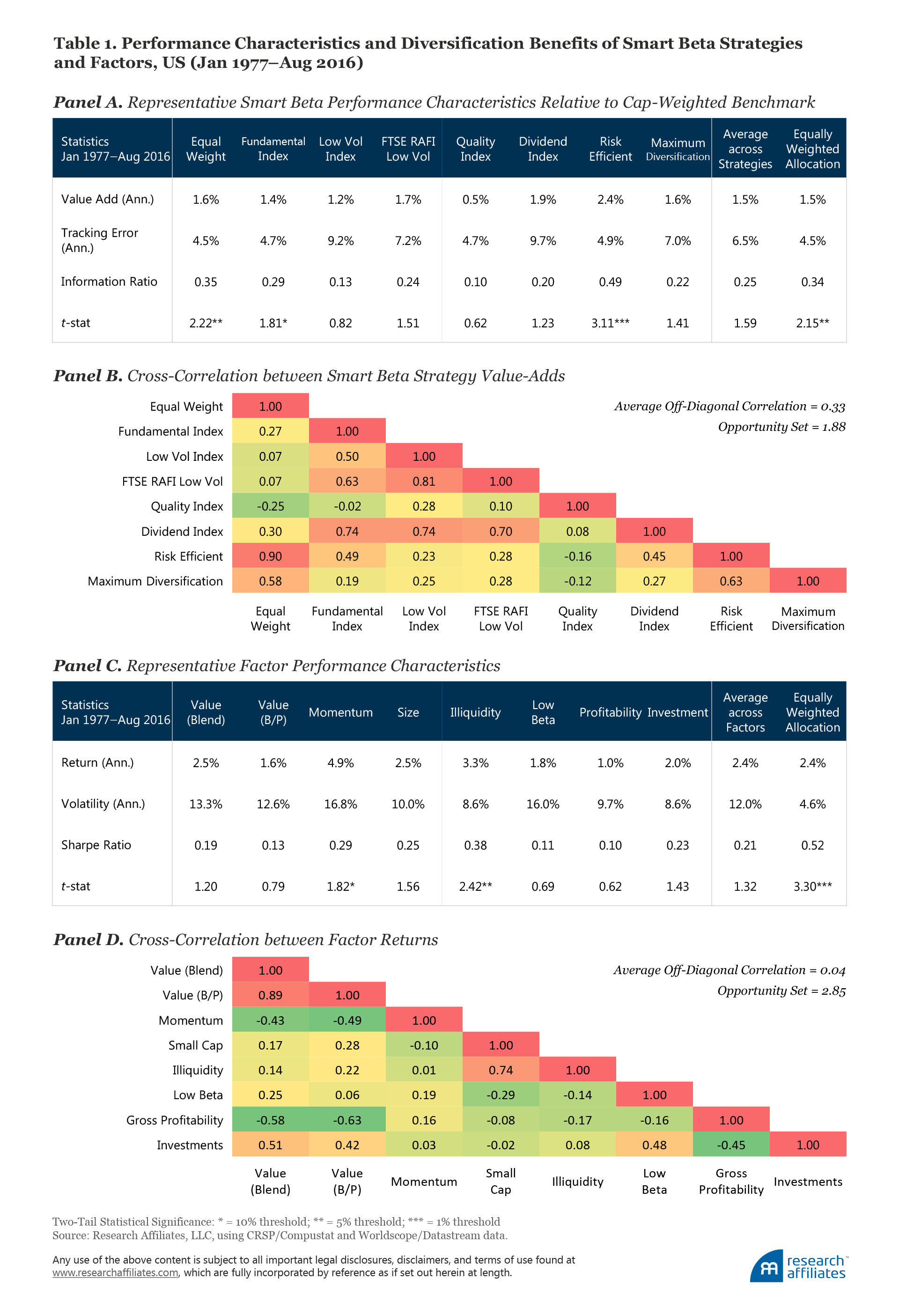
In our replications of smart beta strategies and factors, we attempt to follow a uniform approach.8 Smart beta strategies are long-only portfolios; we display their performance relative to the capitalization-weighted benchmark. By contrast, each factor represents a long–short portfolio. Our long portfolio holds the 30% of the market with the most desirable attributes based on that factor definition, and the short portfolio holds the 30% of the market with the least desirable attributes; both are taken from the large-cap universe. (The exact methodology is provided at the end of the article). For the factors, the performance is the difference between the long and the short portfolios. We display in Table 1 their key performance characteristics. We have not made any adjustments for trading costs, fees, implementation shortfall, or other elements of slippage.9
Our “Straw Man”: Equal Weighting Smart Beta Strategies and Factor Tilts
We set up a straw man, or base-case strategy, in our analysis as hypothetical equally weighted portfolios of the eight smart beta strategies and of the eight factors. In addition to displaying the return characteristics of the individual strategies, Panels A and C of Table 1 also show the return for the straw man portfolios. Not surprisingly, the equally weighted factor-allocation portfolio has a return equal to the average of the eight (1.5% for the smart beta strategies and 2.4% for the factors), but with lower risk, 4.5% versus 6.5%, for the smart beta strategies, and much lower risk, 4.6% versus 12.0%, for the less correlated factors. This means the information ratio for an equally weighted blend of smart beta strategies and the Sharpe ratio for an equally weighted blend of factors are each considerably better than for most of the individual factors and strategies, clearly demonstrating the benefits of diversification. If only we’d had the prescience in 1977 to choose these factors and strategies!
Panels B and D of Table 1 display the correlations between the individual smart beta strategies and factors. Note that although the average cross-correlation of the factors is close to zero (0.04), the two versions of value are highly correlated with each other (0.89). The same is true for the smart beta strategies. Although the average cross-correlation is 0.33, high correlations are observed between strategies.10 Because the factors and strategies are correlated with each other, the number of totally independent factors or strategies is lower than eight. We find a greater opportunity set among factors than among smart beta strategies, which means we would expect any active timing to produce larger effects when implemented across factors—effects which could be for better or for worse.11
Active Timing in Factors and Smart Beta Strategies: The Good, the Bad, and the Ugly
Consider a trend chaser who invests in the three (of eight) smart beta strategies (or factors) having the best blend of 1-, 3-, 5- and 10-year performance at the beginning of each year. This hypothetical rule is a very rough caricature of the way many investors actually invest.
Before going further, however, we would like to stress we’re not advocating a simple reliance on the three cheapest factors or three cheapest smart beta strategies measured relative to their own historical valuation norms, let alone concentrating bets in the one or two cheapest factors or strategies we test. We’re demonstrating that even a simple approach that invests in a lightly diversified roster of three worst performing or least expensive factors or strategies can beat a naïve approach that equally weights all factors or strategies. The strategies are used 1) to illustrate that contrarian investing works across factors and smart betas, 2) to show that trend chasing in factors and smart betas creates a performance drag, and 3) to explore the tradeoff between factor timing and factor diversification.
Figure 1 shows the performance characteristics of an approach that buys the three best performing strategies each year, as well as the performance characteristics of the equally weighted blend of all eight strategies or factors, and a contrarian approach that buys the three worst-performing strategies, also based on a blend of 1-, 3-, 5- and 10-year performance.
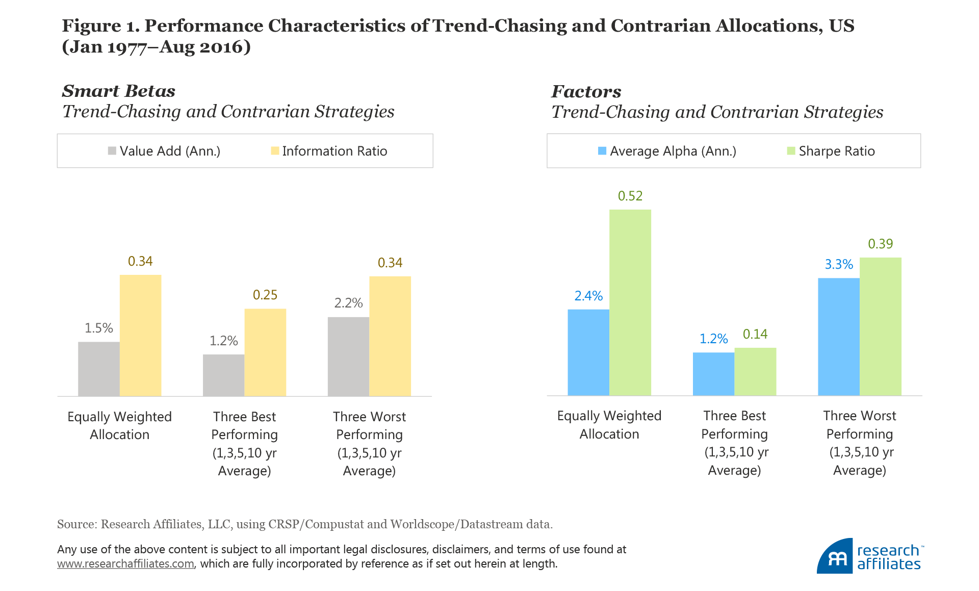
Selecting the three smart beta strategies with the best past performance would have cost the trend-chasing investor 30 basis points (bps) of value-add (1.2% versus 1.5%) compared to sticking with the average smart beta strategy through thick and thin. In the case of factors, the trend chaser loses half of the excess return (1.2% versus 2.4%) relative to the average factor. With the reduction in value-add comes an increase in risk because of the concentration in three (versus eight) strategies. Our smart beta trend chaser suffers a drop in information ratio from 0.34 to 0.25, and our factor trend chaser’s Sharpe ratio plummets from 0.52 to 0.14. Trend chasing, even sensibly using up to 10 years of history to choose our strategies, demonstrably destroys value, even as it increases risk.12
Now, let’s see how our contrarian investor fares. In the case of the smart beta strategies, the contrarian bests the trend chaser with a materially higher value-add (2.2% versus 1.2%) and an improved Sharpe ratio (0.34 versus 0.25), and also performs well against the equally weighted allocation in terms of value-add (2.2% versus 1.5%), while maintaining the same information ratio (0.34) despite less diversification. In factor investing, our contrarian investor has a slightly different result, earning a higher return (3.3% versus 1.2%) and Sharpe ratio (0.39 versus 0.14) compared to the trend chaser, but although value-add is higher (3.3% versus 2.4%) compared to the equally weighted portfolio, the Sharpe ratio is lower (0.39 versus 0.52) due to lower factor diversification and higher risk. The tradeoff between performance and Sharpe ratio will drive different decisions for different investors. For example, we would accept a small haircut in Sharpe ratio in order to earn a materially higher return.
To explore whether our result is a random outlier, we examine the selection rule based separately on past performance over each of the time spans (1, 3, 5, and 10 years) used to form the trend-chasing and contrarian strategies. Panels A and C of Table 2 show the performance results of both the smart beta strategies and factors are largely in line with our earlier result. Every trend-chasing strategy underperforms equal weighting, with a lower information or Sharpe ratio. All the contrarian strategies beat the trend chasers on both performance and information or Sharpe ratio, and all of the contrarian strategies outperform the equally weighted average strategy, although sometimes with a lower Sharpe ratio. The result of contrarian beating equally weighted, which beats trend chasing, holds true in the case of both smart beta strategies and factors, regardless of whether we are looking at 1, 3, 5, or 10 years of past performance.
Many factors and strategies are developed based on long-term data spanning 10 or 20 years. Selecting a strategy based on 10-year results would seem an act of patience and deliberation, hardly a behavior associated with performance chasing. Indeed, seeking the worst performing strategies on a 10-year basis could seem reckless, if not bizarre. And yet, the worst performing beats the best performing rather soundly: 2.0% versus 0.9% for the smart beta strategies and 4.1% versus 1.7% for the factors. The conventional way to use 10-year results—favoring the long-term winners and shunning the long-term losers—is a path to disappointment.
We can’t help but notice that adopting factors or strategies with the best three-year performance produces the worst outcome across all time periods, while embracing factors and strategies with the worst three-year performance delivers the best outcome. Interestingly, consultants and investors often use a three-year period in strategy evaluation and manager selection. Is this the opposite of what should be done? So it might seem.
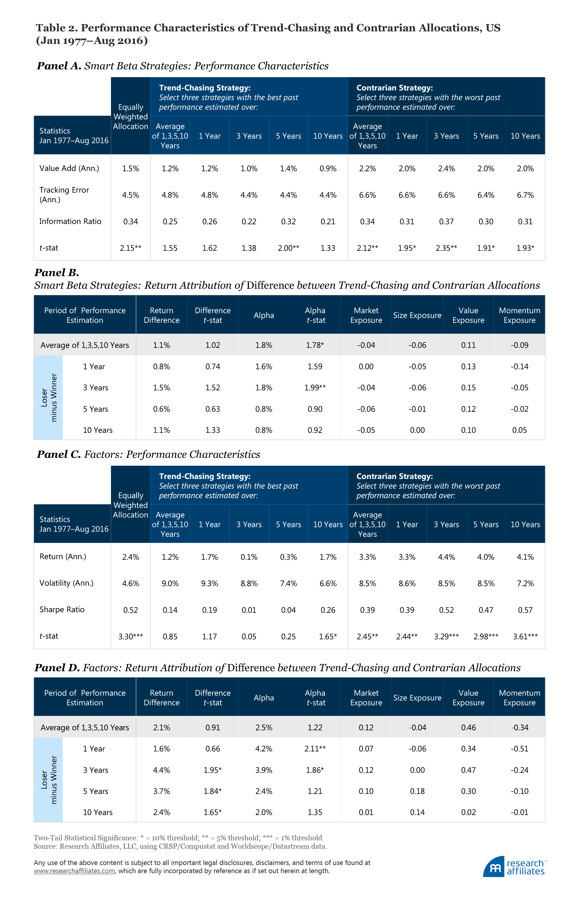
The data in Panels B and D of Table 2 allow us to examine the difference in performance between the contrarian and the trend-chasing strategies in more detail. The difference is material on all horizons and again the biggest difference is at the three-year horizon: 1.5% for smart beta strategies and 4.4% for factors. Is the return difference driven by a systematic bias, favoring one or more of the factors? Is the contrarian strategy just ramping up the value tilt?
Panels B and D also show the results for the Fama–French four-factor attribution of the returns. The difference between the contrarian and trend-chasing strategies seems to have reliably positive value loading and negative momentum loading. But the most interesting result is that, when controlling for the average factor exposures, the return difference is mostly alpha, net of Fama–French factor tilts. Perhaps, surprisingly, the Fama–French four-factor alpha is even larger than the simple return difference in more than half of the cases.
What’s Going On?
Readers of the first two articles in this series know the answer. Valuations matter!
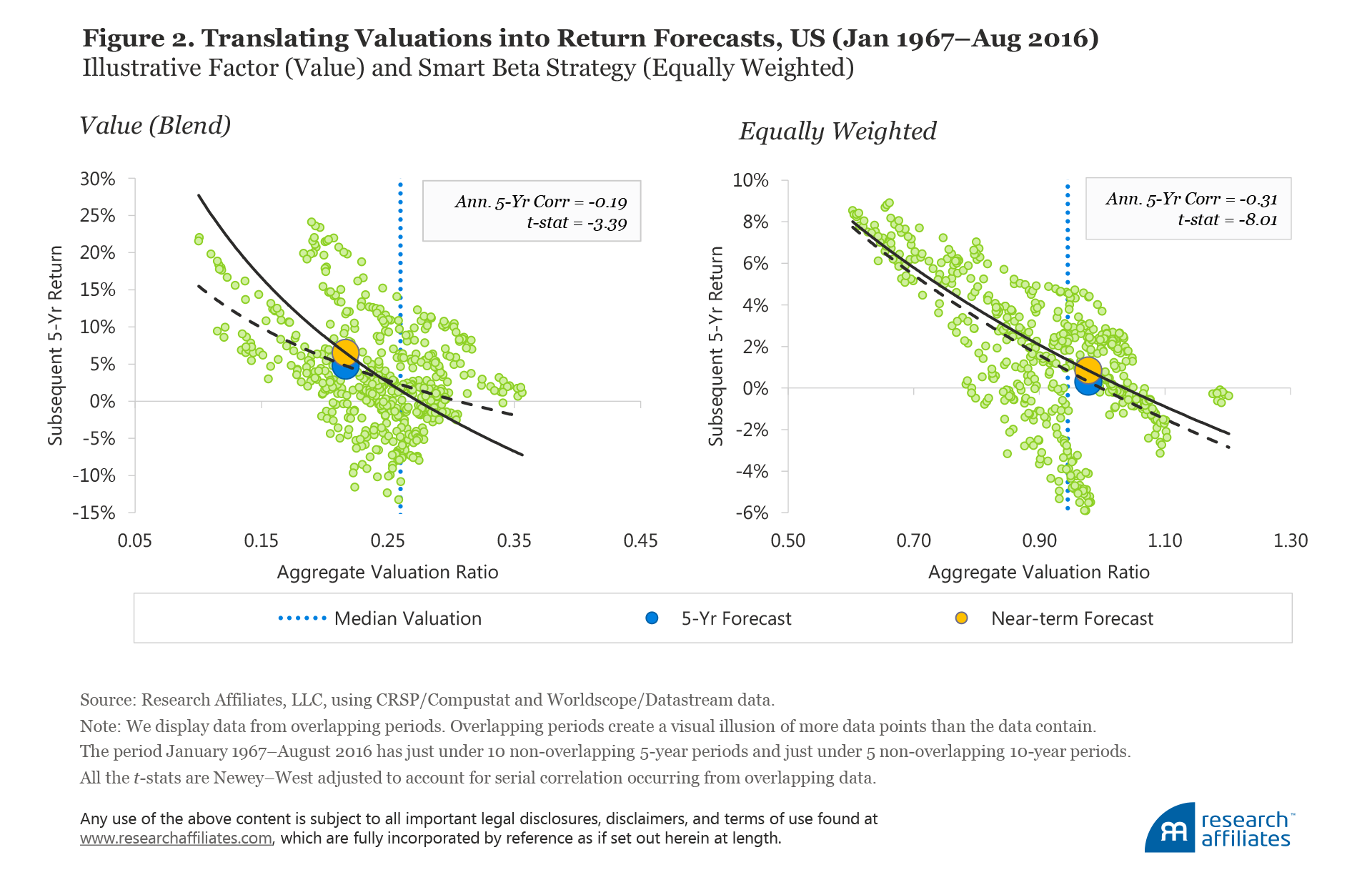
In Figure 2,13 we plot the relative valuations and subsequent performance, spanning nearly a half-century, for the blended value factor and the equally weighted smart beta strategy. Relative valuation measures, for the value factor, how expensive the long side is compared to the short side, and for the equally weighted strategy, measures relative to the market.
We use an aggregate valuation measure that averages four relative valuation metrics—price-to-five-year-earnings, price-to-five-year-sales, price-to-five-year-dividends, and price-to-book ratios—with each measured relative to the cap-weighted market multiple. Figure 2 clearly demonstrates the negative relationship between relative valuation and subsequent performance. In our second article we demonstrate that this relationship between valuation and subsequent return is powerful, robust, and global for almost all factors and strategies in the US, developed ex US, and emerging markets.
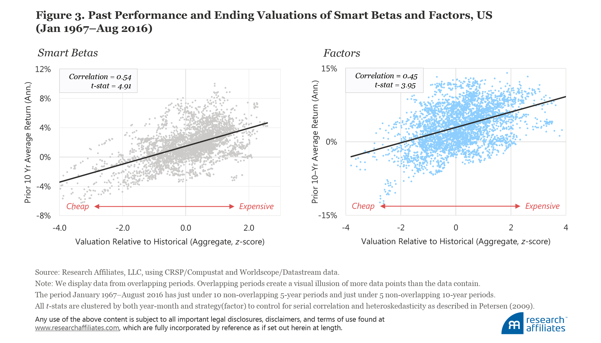
The scatterplot in Figure 3 combines the past performance and relative valuation (versus its respective historical norm) of all eight strategies and all eight factors. The two variables are demonstrably linked with correlations of 0.54 for the smart beta strategies and 0.45 for the factors. When factors or strategies perform well, it’s often because they are getting expensive, while strategies that underperform become cheap based on their relative valuations. The trend-chasing investor would inadvertently select the factors or strategies that have become expensive and this would lead to subsequent underperformance. Investors who select active managers based on past performance are timing strategy and factor selection, but are doing so in a self-destructive way.
Timing Smart Beta Strategies and Factors: Horribly Wrong to Beautifully Right
Our two previous articles, in examining the relationship between relative valuation and subsequent performance, use data from an in-sample test, which tacitly assumes we know all the future norms for relative valuation. Let’s now rid ourselves of this look-ahead bias and see if we can benefit from relative valuation based on prior historical norms.
Each factor or strategy has a different average level of valuation; for example, value factors and strategies are always priced at discounted valuation levels, whereas quality and profitability almost always command premium multiples. More specifically, the Fama–French value portfolio trades, on average, at about one-fifth the price-to-book ratio of growth companies. And quality, defined as the one-third of the stock market with the highest profit margins, typically has an average price-to-book-value ratio about triple the price-to-book of the one-third lowest-margin companies. (So, when price-to-book of high-margin companies is twice the price-to-book of low-margin companies, about one-third cheaper than normal, we would argue that a quality tilt favoring high-margin businesses is likely to be unusually profitable.)
To make relative valuations comparable between factors, we determine the difference between the current relative valuation and the historical average of the relative valuation (available up to any point in history) for each factor or strategy. We then standardize the relative valuation by dividing this difference by the standard deviation of the variations in the past valuations.
Consider an investor who, in the beginning of each year, selects three strategies or factors with the least expensive (cheapest) valuations relative to their own history available to that point. Figure 4, Panel A, shows the performance associated with this approach in the US market from January 1977 to August 2016. The figure also presents the results for the three most expensive strategies and factors as well as the performance of the equally weighted mix of factors and strategies.
An investor in the three cheapest smart beta strategies would have outperformed an investor in the equally weighted strategy by about 0.5%. This may not seem a large margin, but over the 39½-year period an investor holding the three cheapest smart beta strategies would have been 108% richer than an investor holding the cap-weighted market, as Figure 4, Panel B, illustrates. By contrast, the investor holding the equally weighted strategy would have been 75% richer than an investor in the cap-weighted market. Even tenths of basis points compound quite nicely over time.
By constantly rebalancing into the cheapest strategies, an investor will rarely be buying the strategies with the most reliable alpha, which will often be the strategies with the largest structural alpha. Imagine how much outperformance can be added by favoring the strategies with a large structural alpha that are also trading cheaply relative to their historical norms!
An investor in the three cheapest factors would have outperformed an investor in the equally weighted factor mix by about 3.7%. Even though the approach has a systematic bias away from the factors with the highest structural alphas, our focus on the cheapest strategies overcomes that headwind, with 370 bps a year of room to spare.
An investor holding the three most expensive factors would have performed worse than the market—even when these factors were chosen for their positive average performance after the fact! For smart beta strategies and factors, the approach of selecting the three most expensive provides a lower return compared to the respective equally weighted mix. Relative valuations predict future premia for both smart beta strategies and factors, and this result holds out of sample.
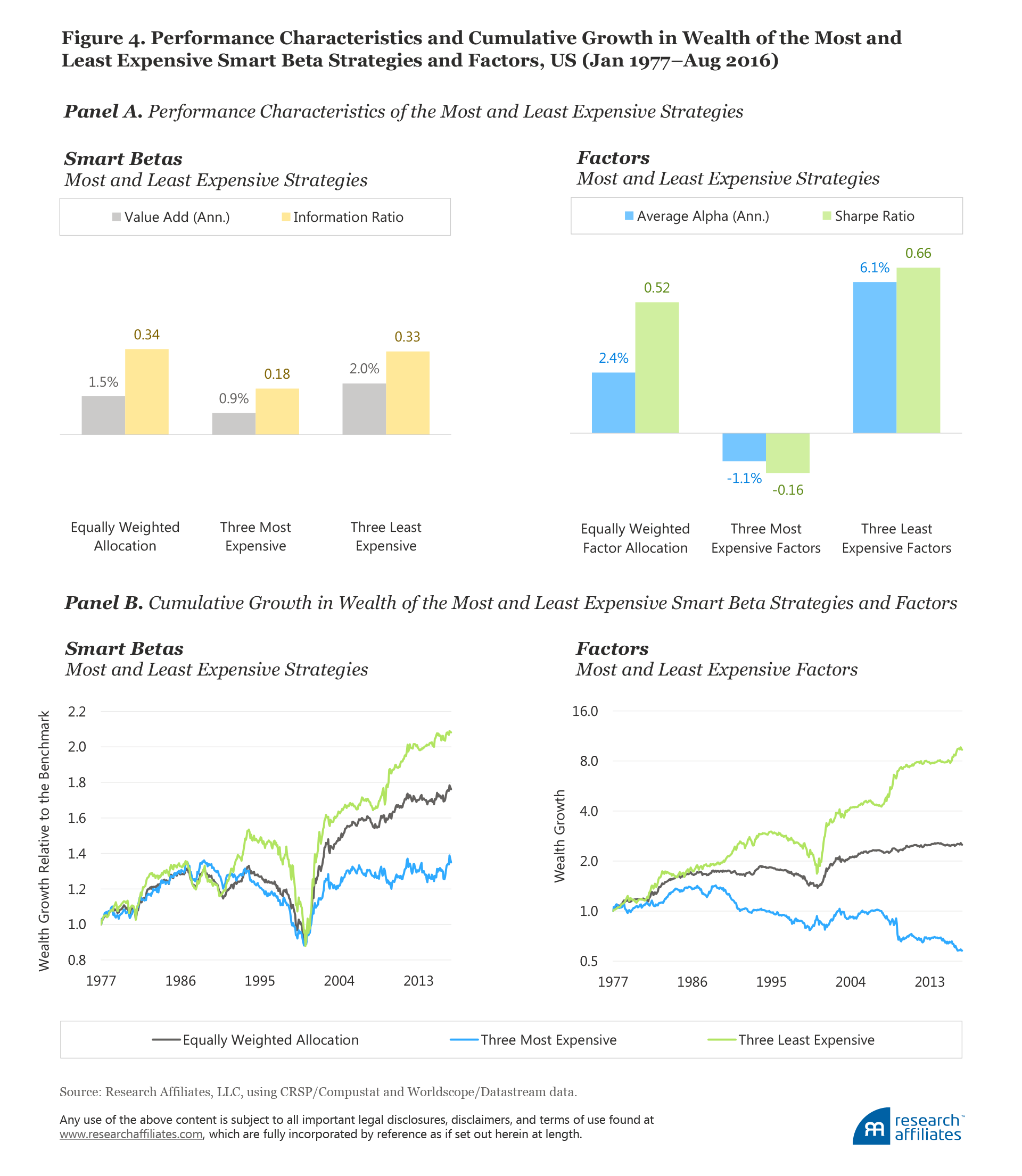
Trend chasing is perceived to be safe—after all, who gets blamed for investing in what has recently done well? We can expose the fallacy of this perception of safety by comparing the cumulative growth of wealth over the last 39½ years for the three approaches—equally weighted, three most expensive, and three least expensive—in Panel B of Figure 4. The more expensive strategies not only deliver poorer performance, but they are unable to offer safe harbor in times of a market crash. The severe drawdown resulting from the tech bubble’s bursting in late 2000 afflicted all three strategies, most particularly for the investor buying the cheapest strategies. Given that the tech bubble was a momentum and growth market, it’s noteworthy it was also a tough time for the strategy that buys the most expensive (and recently successful) smart beta strategies and factors.
Isn’t This Just Value Investing on Steroids?
Charlie Munger has said “All intelligent investing is value investing—acquiring more than you are paying for.” So, if we’re emphasizing the cheapest factors and strategies relative to their own history, are we doubling down on value? Yes and no. The approach tilts factor allocation to the factors cheaply priced today, relative to their own histories, and is not the same as doubling down on the value factor. Relative valuations can lead us to invest in the value factor when value is cheaply priced and to avoid value and invest in other factors when value is richly priced. Tilts are based on which factors or strategies are cheap relative to their historical norms, not simply steroid boosting the value tilt.
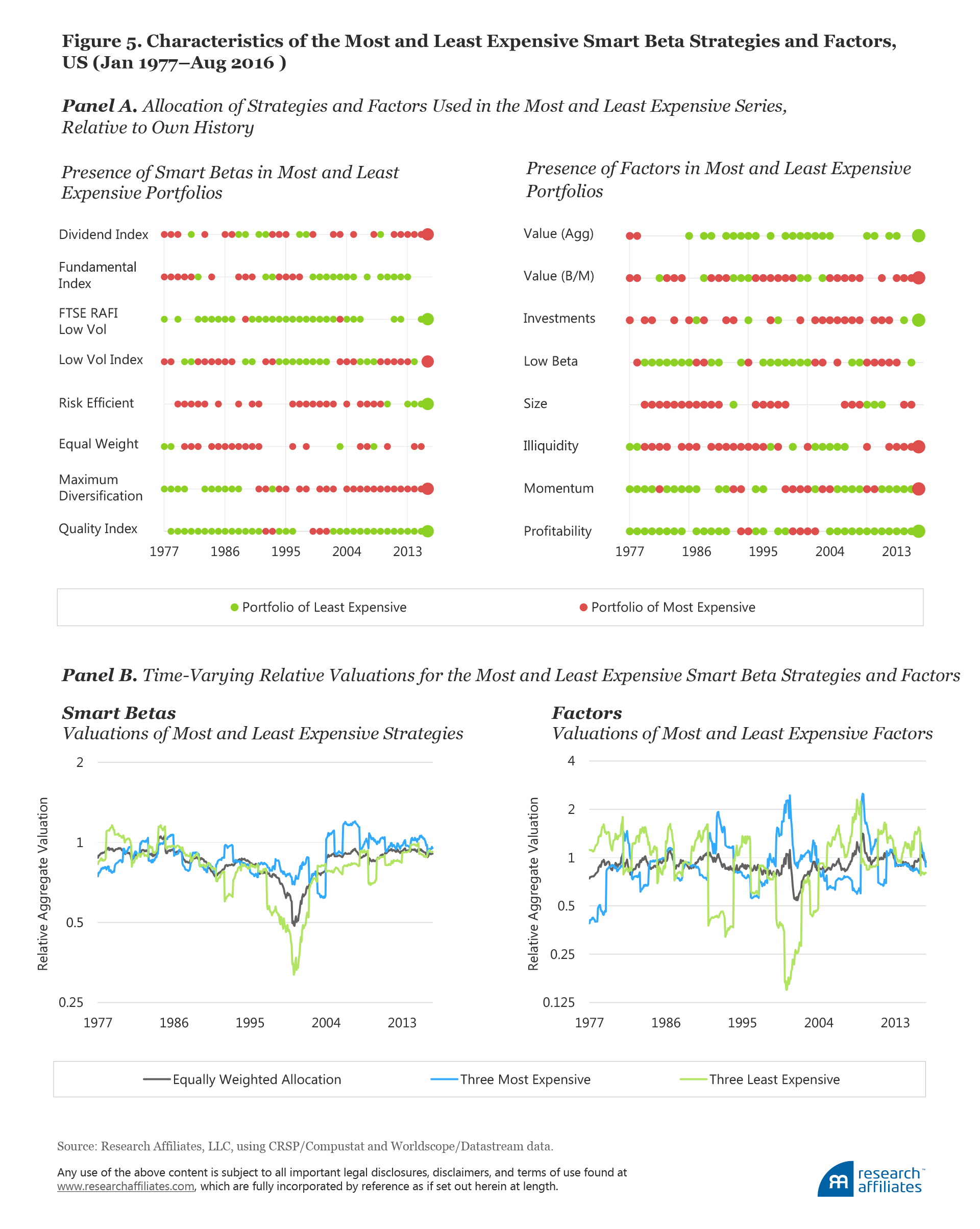
Every one of the eight smart beta strategies and eight factors finds its way into the least expensive portfolio on multiple occasions over the 39½-year period, as Panel A of Figure 5 illustrates. This figure shows, year by year, which strategies and factors make their way into the cheapest three (green dots) and most expensive three (red dots) portfolios. The final dots show the portfolios created for 2016. The portfolio which relies on the least expensive strategy is not boosting the value tilt, per se, but is strategically shifting allocations in a contrarian manner. These (admittedly simplistic) timing strategies move into value when value is cheap and into growth-oriented factors, such as momentum and profitability, when they are cheap.
Figure 5, Panel B, offers another way to assess the actual value tilt of the strategy. Often the “inexpensive” strategies and factors—relative to their own history—are more expensive than the “expensive” strategies. In other words, when value is expensive relative to its own history, it will be in the portfolio of expensive strategies, even if it’s always cheap relative to the market or relative to growth. Our focus on the inexpensive factors and strategies can, perhaps surprisingly, lead to a growth tilt, nearly as often as it leads to a deeper value tilt.
The performance difference between the three cheapest factors and the three most expensive factors in the US market, reported in Panel B of Table 3, was 7.2% a year over the period from January 1977 to August 2016. With a t-statistic of 3.62, the difference is highly economically and statistically significant.14 In international markets, the difference is far smaller and not significant, which is perhaps a consequence of currently stretched factor (and smart beta) strategy valuations in non-US markets. If these markets mean revert, the gap (and its significance) will presumably rise. Interestingly, even with the stretched valuations, buying the cheaper strategies and factors would have proved beneficial.
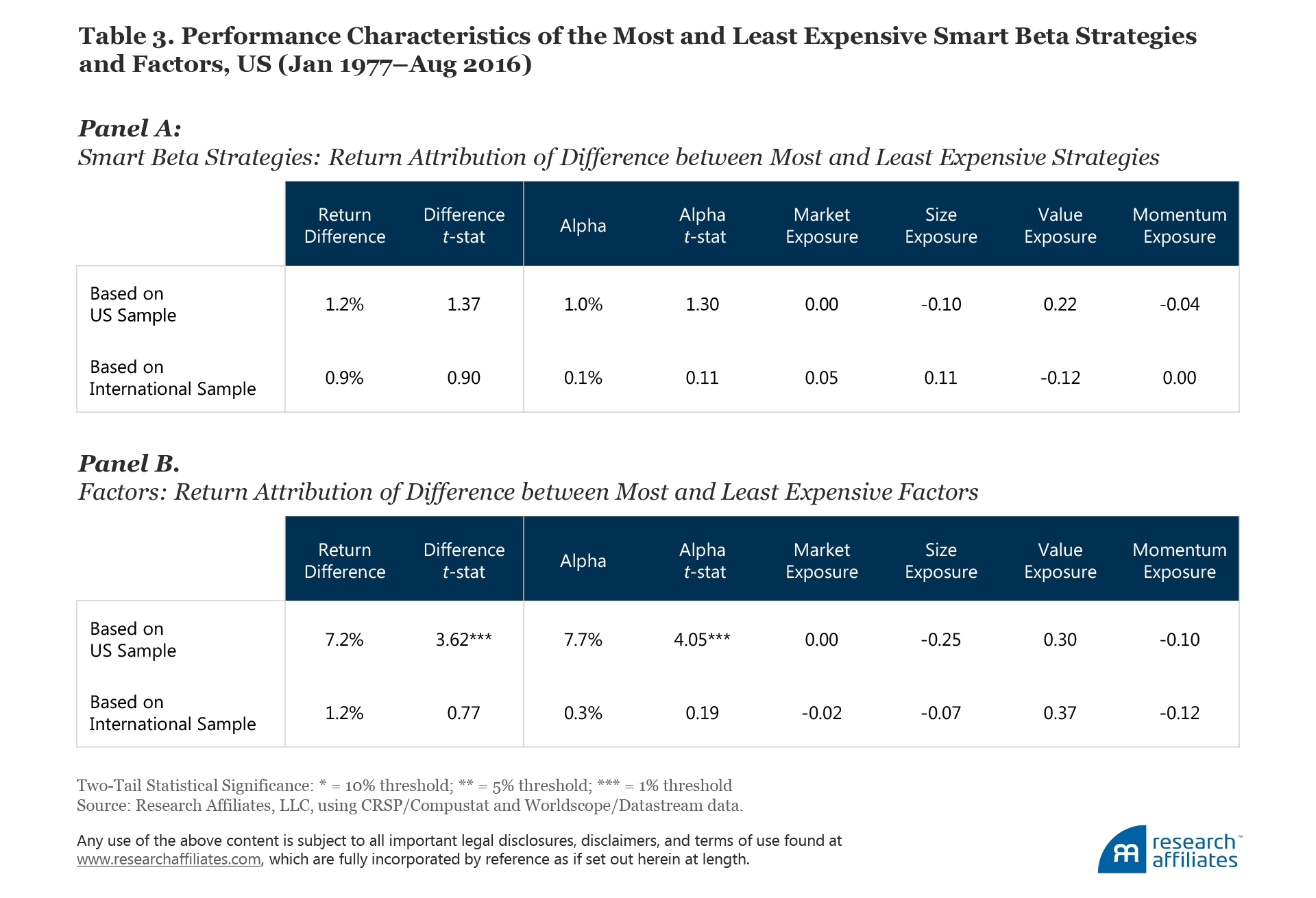
The return attribution to the Fama–French plus momentum four-factor model, reported in Table 3, shows the return difference between the cheapest and the most expensive strategies (both US and international) has a positive, but unreliable, loading to the value factor (in three of four cases). Similar to the data reported in Table 2, Panels B and D, we note, with some surprise, that the largest source of return from active timing of factors or smart beta strategies is attributed to alpha, net of—and not explained by—the four factors. The performance difference is not explained by value risk loading.
We’re All Data Mining!!
Investors, academics, product innovators—all are data mining. In our analysis even we are data mining. All of the eight smart beta strategies we test outperform their cap-weighted benchmark and all of the eight factors we test have positive returns. No surprise because we examine the most popular strategies and factors, and their popularity is driven by good past performance.
Of course, most new strategies begin with a backtest. This is not a bad thing as long as the alpha can be credibly explained by economic theory, behavioral finance, or at least some financial intuition. Today’s multi-strategy and multi-factor programs are typically sold and embraced as if none of this data mining is taking place. But it is. Note that backtested performance is not an ideal basis for shaping expectations, especially if we do not disentangle structural from revaluation alpha; in the past, this step has been routinely ignored.15
Our straw man, an equally weighted roster of eight factors or eight smart beta strategies, none of which were investable over the entirety of the last 50 years, suffers from a rather extreme form of data mining: our tests tacitly pretend these strategies and factors were all known and investable in 1977.16 For example, Standard & Poor’s created its equally weighted index in 1990, the Fundamental Index™ was launched in 2004 as a strategy and in 2005 as a published index, and so forth. As for the factors, value was first published in 1977, size in 1981, and so on.
We (like the rest of the investment community) are also subject to selection bias. The factors and strategies in our straw man could not have been chosen in 1977, 1987, or even 1997, decades that are included in our study. That’s data mining. Can our tests include factors or strategies that have yet to be discovered? Of course not. Were there factors, anomalies, and strategies discovered in the early decades of quantitative finance that have fallen out of favor because of disappointing subsequent performance? Of course. Are these included in any of our tests, or any of the commercially available multi-strategy programs? Of course not.
Our tests of the adoption of recently disappointing strategies or of the cheapest strategies relative to their own historical norms (i.e., a contrarian approach) does not rely on look-ahead bias, and therefore is not subject to the worst forms of data mining. Even so, we would not be surprised to find less incremental alpha from a contrarian reliance on cheaper strategies than our own tests would indicate.
Measuring the Impact of Data Mining from Academic “Factor Timing”
Investors are hardly the only factor timers. Academics and product innovators are timing right along with investors. We’re huge fans of product innovation, but there’s good news and bad news in the product proliferation that results. The good news is investors have a far richer toolkit than in the past: today many low-fee strategies permit investors to build a portfolio to match their needs. The bad news is too many investors use this panoply of choice to chase the strategies with the best past performance rather than checking which strategies are trading cheaper than their historical norms, and therefore may offer better future returns.
Academics have been looking at factors for a number of decades now. Indeed, the “new” factor-tilt approach to investing dates back to the early 1990s, if not earlier. In academia, publications and citations beget tenure and academic success, strong incentive for the “discovery” of yet another new factor—and each one has strong past performance.17 Why would an author submit a paper exploring an idea that loses money? Why would a journal have any interest in printing such an article?
Newly launched products are, not surprisingly, based only on indices, strategies, and factors with positive backtested returns.18 We mine data to find ideas that (historically) work. We publish and build products only on those with noteworthy profitable results. There’s no wickedness involved here; all of us are genuinely seeking the best ideas from the past, tacitly presuming that past is prologue. Those who invest in these ideas are wise to be skeptical and to give touted performance numbers a haircut: a light one for very simple ideas that are not heavily data mined and a much heavier one for profoundly data-mined ideas that are carefully fit to historical data.
We can, albeit with very poor precision, measure the “phantom alpha” of new factors. Our analysis looks at how the smart beta strategy or factor fares after it was discovered, and how those results compare with the results that brought attention to the idea in the first place. Table 4 presents our findings. The average excess return of the smart beta strategies (Panel A) before index launch is 1.8%. After launch the average excess return is 1.4%, or 0.4% lower. The average excess return of the factors (Panel B) before publication is 5.8%, and after publication only 2.4%. On average, about 22% of the smart beta alpha, and over half of the factor alpha, evaporated after launch or publication. Six of the eight factors produced lower returns after they were published.
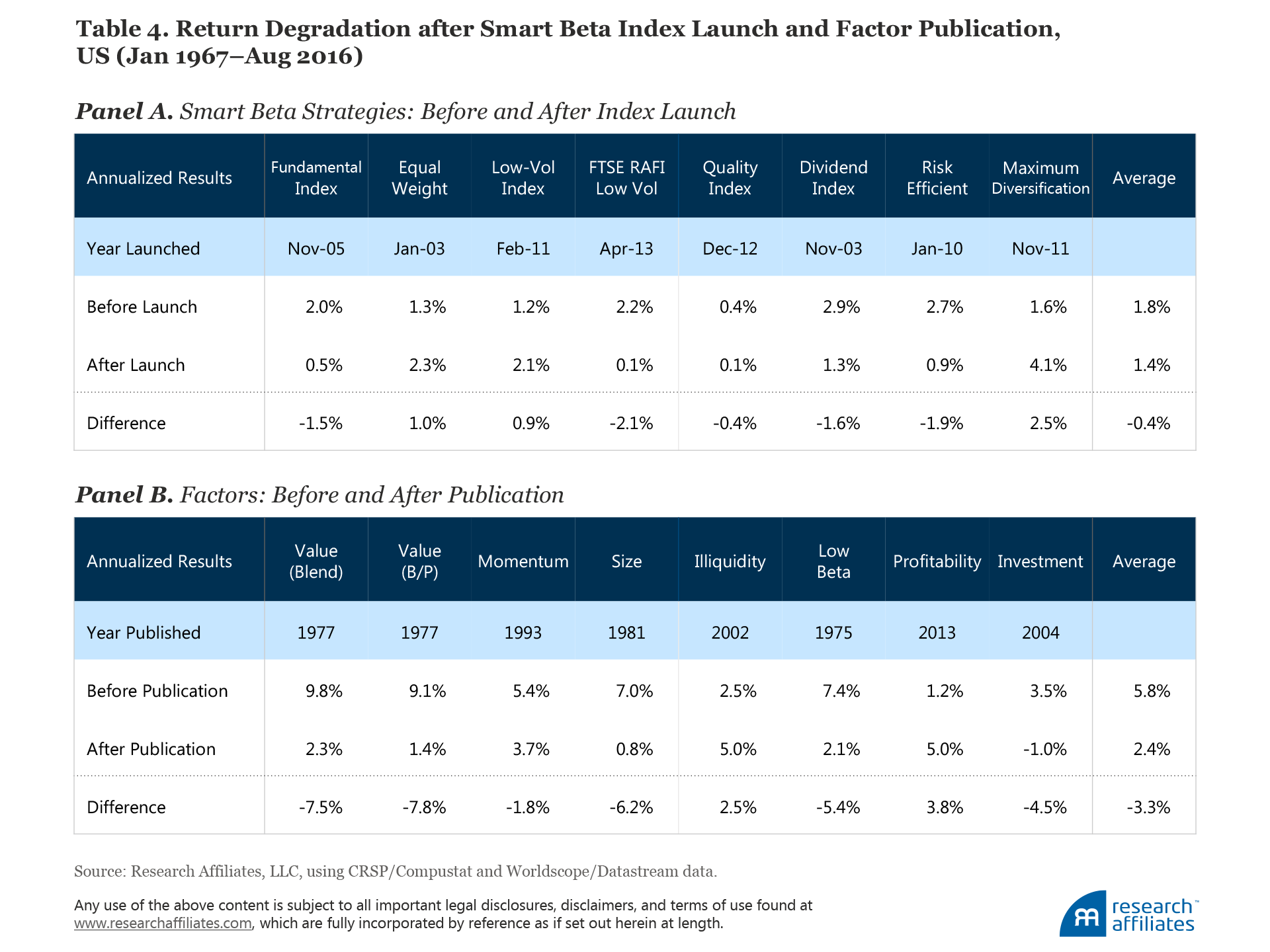
Some of the lower performance after publication or index launch can be explained by in-sample bias: it is easier to notice, and to publish, a strategy or factor that has delivered statistically significant past performance, even if that success was luck (or upward revaluation). Another reason for the performance difference is, no doubt, arbitrageurs trying to profit from the newly publicized source of better performance. Lastly, and very likely, the strong past returns that caught the interest of academics included revaluation alpha from rising relative valuation multiples. Thus, academics discover factors when they are expensive, which drives their prospects for future returns down.
The fiduciary standard may pull us even further toward performance chasing. Although it may be profitable to invest in a factor or strategy with miserable past performance, the decision could be quickly branded “imprudent” whenever the investment inevitably fails to add value. Consultants, RIAs, and financial advisors are obviously reluctant to advise a client to invest in a newly cheap strategy or factor, knowing they could be successfully sued if it doesn’t work. Given that chasing past performance may be a good way for fiduciaries to avoid the label of imprudence, even if one of the worst ways to add value, we believe our findings may actually understate the future efficacy of contrarian investing in a world that ever more reliably shuns bargains.
Measuring the Impact of Data Mining from International Evidence
Another way to gauge—again crudely—how much error is introduced by data mining is to go “out of sample” by looking at results using international data. Most of the smart beta strategies and factors were identified in the US stock market. As we explain in “To Win with ‘Smart Beta’ Ask If the Price Is Right,” the factors work less well outside the United States, with the exceptions of value and momentum. Some academics and practitioners respond to this challenge by trying to modify the factors so they will work better outside the United States. They are, of course, data mining! Most of the smart beta strategies “export” well: most work as well, if not better, outside the United States as in the original US results.
Table 5 offers a more detailed look at the performance characteristics of the least expensive and most expensive strategy portfolios in the United States and developed ex US markets. Both the smart beta strategies and the international samples have slightly weaker results compared to the factor results in the United States. In all cases, however, a material difference exists between the least and the most expensive strategies and factors. The contrarian, or least expensive, approach also wins internationally, albeit by a smaller margin than in the United States.
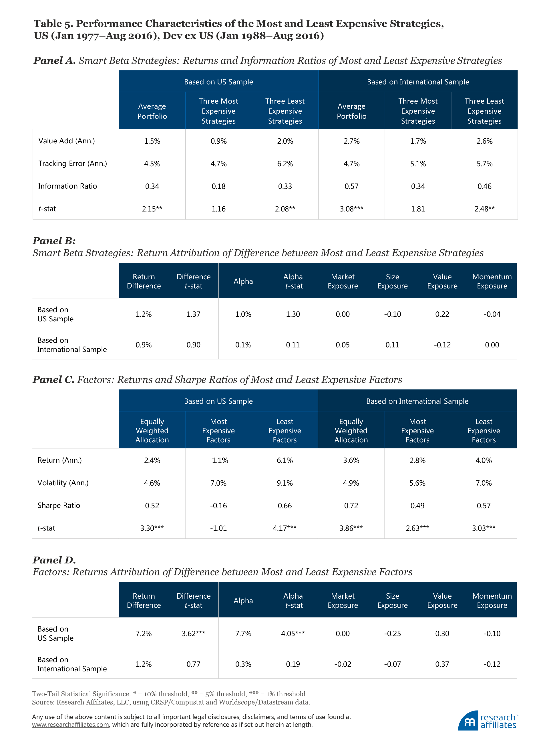
In addition to US data mining, we would expect the international results to be weaker than the US results for a couple of reasons. Contrarian strategies profit from mean reversion, but mean reversion is a more powerful tool when we have an accurate fix on the “mean” we are reverting toward! The international results span a shorter time frame than the US results, so the available estimate of the historical relative-valuation norm for each strategy or factor outside the US market doesn’t allow us to gain a reasonably accurate gauge of the mean.
Also, the non-US markets have experienced a tremendous flight to safety since the global financial crisis. As a result, many factors and strategies—notably those viewed as less risky, such as quality or low beta—are trading at stretched valuations, far more so than in the United States. In this environment, it’s actually a pleasant surprise that contrarian investing has been at all profitable outside the United States, as it would have bought the out-of-favor stocks (which are still out of favor!) hurting performance in recent years. Are the non-US markets experiencing a “new normal” or are they past-due for mean reversion? No one can know the answer, but based on past experience, the latter seems more likely. It will be interesting to re-examine these results in a few years when current factor bubbles (if that’s what they are) have had an opportunity to mean revert toward their respective historical valuations.
The return difference is lower among smart beta strategies than among factors for two reasons. First, the factors are 100% long and 100% short; the active share (or the difference between the two portfolios) is 200%. In contrast, the smart beta strategies have considerable overlap because of their cap-weighted benchmarks; the active share is typically 30–60%. Second, the smart beta strategies are more highly correlated, as we showed in Table 1, than are the factors, whose average correlation is near-zero. Consequently, combinations of smart beta strategies are much more alike than combinations of factor tilts. When the relative valuation signal is applied to selecting the most and least expensive factors or strategies, factors offer more breadth, and therefore, experience a stronger impact from timing compared to the smart beta strategies. We observe the same effect outside the United States.
Conclusion
Can investors time markets, factors, and strategies? Our answer is not only “yes, they can” but almost everyone is already doing so, often without realizing it. Unfortunately, most investors are factor timing in the wrong way by chasing past performance, similar to the temptations many face in manager selection and asset allocation.
We use a simple rule to show that trend chasing destroys value. Whatever is newly expensive is likely to have two attributes: wonderful past returns and disappointing future returns. Whatever is newly cheap is likely to have the opposite attributes: lousy past returns and solid future returns. Human nature causes us to anchor on those past returns in shaping our expectations for the future. No wonder we’re all tempted by performance chasing.
The so-called smart beta revolution has led to impressive innovation and to breathtaking product proliferation, a situation both wonderful and dangerous. Products are being offered based on wonderful backtests. The mere act of embracing a new strategy with strong recent results—and likely higher valuations than historical norms—is a tempting and pernicious form of performance chasing.
Investors who choose to invest in strategies with the better past (and often recent past) performance hurt themselves, especially when they do so without asking whether the strategy (or asset class or factor) delivered that past performance merely by becoming newly expensive and whether the strategy is trading at dangerous valuation levels. Some practitioners counsel against asking these questions. We find this advice disturbing.
We show that trend chasing—even when diversifying among three factors with the recent strongest results, and even with a cherry-picked set of strategies that have performed well over the half-century span we test—can destroy the benefits of factor investing. If we had any way to eliminate the data mining and selection bias and to conduct a true out-of-sample test, results could only be worse for trend chasing (and admittedly, the benefits from contrarian trading of strategies might also be less than the results we show here). If investors swing into smart beta strategies and factor tilts that today have wonderful 5- and 10-year alphas without asking whether they are newly expensive, and those alphas reverse in the years ahead, smart beta investing could go “horribly wrong.”
Today, currently stretched relative valuations provide a smart beta/factor investing opportunity, that when used intelligently, can instead be “beautifully right.” Selecting strategies with sound structural alpha—sound performance when controlled for rising valuation multiples—currently trading at a discount to historical norms may deliver performance higher, not lower, than the backtests. Smart beta is crowded space, consisting of some good ideas, some not-so-good ideas, and some good ideas that are temporarily overpriced. Look before you leap!
Endnotes
- We previously used the term “situational alpha,” but others have suggested “revaluation alpha,” which we rather like better than our own nomenclature! We’re embracing the change in terminology in this third article of our series.
- We do not mean this in any pejorative way. We’re all data miners, even if inadvertently, merely in the act of seeking ideas that can add value. While there’s (usually) nothing nefarious about it, we owe it to ourselves and to our clients to acknowledge we’re engaged in data mining and to try to minimize the extent our decisions rely on it.
- As we’ve shown in previous articles, factor tilts explain most of structural alpha. This is not to say these alphas could be recreated with factor tilts! As we’ll explore in a future article, factor-tilt strategies deliver factor alpha minus implementation shortfall. The fact that smart beta strategies mostly have alpha, over and above the alpha explained by factor tilts, is actually a huge “win.”
- Value investing first appeared in the academic literature in Basu (1977).
- We distinguish between factor tilts and smart beta strategies for reasons outlined in Arnott and Kose (2014). We’re clearly losing this battle as the term “smart beta” is stretched to encompass factor-tilt strategies and a host of ideas, some smart, some not smart. If the term smart beta encompasses almost everything, then the term means nothing.
- We examine the Fundamental Index™, an equally weighted index, a low-volatility index, the FTSE RAFI™ Low Volatility Index, a quality index, a dividend-weighted index, a risk-efficient index, and a maximum-diversification index.
- We examine value (Fama–French HML), low beta, gross profitability, momentum (UMD), size (SMB), illiquidity, and investment. As a robustness check we test two versions of value. One is constructed using the price-to-book ratio (the most common academic definition of value), and one is based on a blend of four valuation metrics: price-to-five-year-earnings, price-to-five-year-sales, price-to-five-year dividends, and price-to-book ratios. With two versions of value we have a total of eight factors which we use as a starting point in our analysis.
- All smart beta strategies are constructed from the largest 1,000 stocks by market capitalization to make comparison less vulnerable to idiosyncrasies unrelated to index methodology. The only exception is the Fundamental Index where, following methodology of Arnott, Hsu, and Moore (2005), we use the top 1,000 names by fundamental measures of company size. With the exception of the momentum factor portfolio, which is rebalanced monthly, all other factors (and all smart beta strategies) are rebalanced annually at yearend.
- Slippage can be huge. The momentum factor has delivered a 5% return (up stocks beating down stocks by 5% a year) since the last momentum “shock” during the global financial crisis. Despite this, we are not aware of any momentum funds that have delivered a positive alpha, let alone 5%.
- On closer examination we find most of the popular smart beta strategies are positively correlated to the Fundamental Index and the dividend index, indications of a strong element of value and small-cap exposure relative to the benchmark. The benchmark assigns weights proportional to company capitalization, overweighting overpriced growth companies and underweighting underpriced value companies. The value exposure almost automatically arises as the byproduct of many smart beta strategies not using capitalization to assign weights to individual stocks.
- The Opportunity Set (OS) is defined by Grinold and Taylor (2009) as
 , where r is the vector of excess returns and Ω is the covariance matrix. While OS is technically the maximum ex post Sharpe ratio that could have been obtained by optimal allocation (in our case allocation across the eight smart beta strategies or eight factors), it is also a useful measure of the effective breadth of a portfolio. Portfolios can achieve breadth and increase their opportunity set by including more assets, especially if they have low correlations with each other. For example, making investment decisions across 10 uncorrelated assets will provide more opportunity for higher performance than with only 5 uncorrelated assets. Likewise, 10 uncorrelated assets will provide more opportunity than 10 assets with correlation near 1.0 (having correlation near 1.0 would be similar to having the breadth of just 1 asset). Similarly, portfolios with more volatile assets have more breadth and a larger opportunity set. For example, 10 volatile assets will provide more opportunity than 10 assets whose prices don’t move; without changing prices, even the most skilled investor could not outperform. We find that our set of eight factors provides more opportunity to take advantage of timing signals than our set of eight smart beta strategies. We, therefore, expect a wider spread between timing well versus timing poorly in factors than we do in smart betas. This is, in fact, exactly what we see.
 - Hsu, Myers, and Whitby (2016) show that investors are measurably destroying value by selling funds at cheap levels and buying at expensive levels. The poor timing of purchases and sales by investors destroys value, resulting in their underperforming the broad market.
- For illustrative purposes, we show two charts from our prior work updated through August 2016. Please refer to the first two articles in this series for a complete set of these analyses.
- This comparison is of the relative valuation of a factor or strategy to its own prior norm with no look-ahead bias. The statistical significance is particularly interesting because this would be expected to degrade the statistical significance, relative to an in-sample test.
- We have fallen prey to this error, too! When Jason Hsu, Philip Moore, and I published “Fundamental Indexation” in 2005, it did not occur to us to test whether RAFI™ was newly expensive at that time or to test if the past performance of RAFI was partly driven by rising valuations. Had we done so, we would have discovered that a modest fraction of the historical alpha of RAFI was revaluation alpha, and that RAFI was trading a little rich at the time. This gives us special satisfaction to observe that RAFI has added value since its introduction, all over the world, despite a headwind of becoming cheaper—much cheaper—over the subsequent decade. We can’t wait to see how it works when it finally enjoys a tailwind from value winning!
- In our earlier articles, our analysis began in 1967. Our current analysis begins in 1977 because we use trailing 10-year performance as one of the selection criteria in our strategy and factor-timing tests. We also use valuation relative to that factor or strategy’s own history; starting in 1977 allows us to start with 10 years of historical valuation data.
- Harvey, Liu, and Heqing (2015) cannot recall in their survey a single published article about a new factor or smart beta strategy that did not reportedly generate alpha.
- According to Brightman, Li, and Liu (2015), ETF providers evidently take investors’ preference for winners into account by predominatelylaunching funds whose underlying indices are outperforming at the time they make new product decisions.
- Beck et al. (2016) provide an examination of factor robustness and implementation costs.
References
Amenc, Noël, Felix Goltz, Lionel Martellini, and Patrice Retkowsky. 2010. “Efficient Indexation: An Alternative to Cap-Weighted Indices.” EDHEC-Risk Institute (January).
Arnott, Robert D., Jason Hsu, and Philip Moore. 2005. “Fundamental Indexation.” Financial Analysts Journal, vol. 61, no. 2 (March/April):83–99.
Arnott, Robert D., and Engin Kose. 2014. “What ‘Smart Beta’ Means to Us.” Research Affiliates Fundamentals (August).
Basu, Sanjoy. 1977. “Investment Performance of Common Stocks in Relation to Their Price-Earnings Ratios: A Test of the Efficient Market Hypothesis.” Journal of Finance, vol. 32, no. 3 (June):663–682.
Beck, Noah, Jason Hsu, Vitali Kalesnik, and Helge Kostka. 2016. “Will Your Factor Deliver? An Examination of Factor Robustness and Implementation Costs.” Financial Analysts Journal, vol. 72, no. 5 (September/October):58–82.
Brightman, Chris, Feifei Li, and Xi Liu. 2015. “Chasing Performance with ETFs.” Research Affiliates (November).
Choueifaty, Yves, and Yves Coignard. 2008. “Toward Maximum Diversification.” Journal of Portfolio Management, vol. 35, no. 1 (Fall):40–51.
Fama, Eugene, and Kenneth French. 1993. “Common Risk Factors in the Returns on Stocks and Bonds.” Journal of Financial Economics, vol. 33, no. 1 (February):3–56.
———. 2012. “Size, Value, and Momentum in International Stock Returns.” Journal of Financial Economics, vol. 105, no. 3 (September):457–472.
Frazzini, Andrea, and Lasse H. Pedersen. 2014. “Betting Against Beta.” Journal of Financial Economics, vol. 111, no. 1 (January):1–25.
Grinold, Richard C., and Mark P. Taylor. 2009. “The Opportunity Set: Market Opportunities and the Effective Breadth of a Portfolio.” Journal of Portfolio Management, vol. 35, no. 2 (Winter):12–24.
Harvey, Campbell R., Yan Liu, and Zhu, Heqing. 2015 “…and the Cross-Section of Expected Returns.” (February 3). Available at SSRN.
Hsu, Jason, Brett W. Myers, and Ryan Whitby. 2016. “Timing Poorly: A Guide to Generating Poor Returns While Investing in Successful Strategies.” Journal of Portfolio Management, vol. 42, no. 2 (Winter):90–98.
Newey, Whitney K., and Kenneth D. West. 1994. “Automatic Lag Selection in Covariance Matrix Estimation,” Review of Economic Studies, vol. 61 (April):631–653.
Petersen, Mitchell A. 2009. “Estimating Standard Errors in Finance Panel Data Sets: Comparing Approaches.” Review of Financial Studies, vol. 22, no. 1: 435–480.
Appendix: Diversification Effects in Timing Smart Betas and Factors
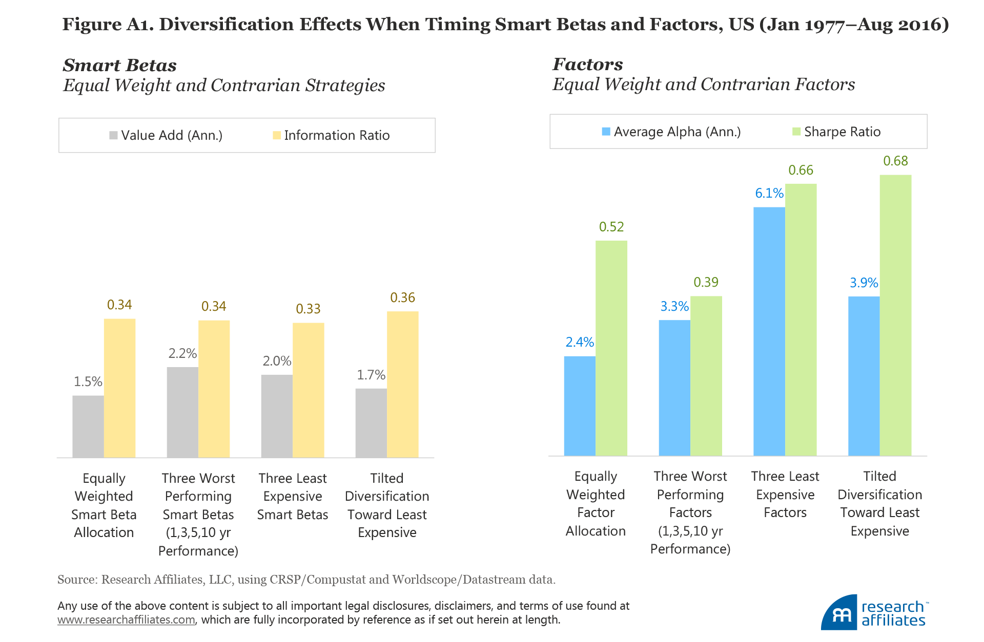
In our analysis of the eight smart beta strategies, we observe that a combination of the three strategies with the most attractive (least expensive) valuations tends to generate a higher return relative to an equally weighted mix of all eight strategies. The higher return does not come with an improvement in the Sharpe ratio because of the loss in diversification relative to the well-diversified equally weighted mix. To further study the benefits of diversification, we simulate one more strategy:
Tilted Diversification toward Least Expensive Strategy: Weight all strategies and factors from the least to the most expensive proportional to 4,4,3,3,2,2,1,1.
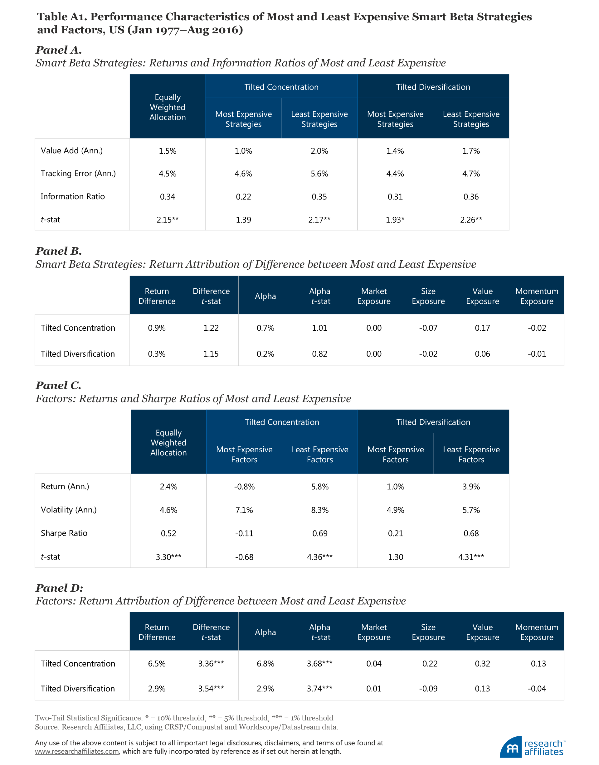
The performance of this strategy is presented in Figure A1. We compare its return and risk to three other approaches: an equally weighted allocation, a contrarian approach combining the three worst-performing strategies/factors, and a combination of the three strategies/factors with the least-expensive valuations. For both smart beta strategies and factors, the tilted-diversification-toward least-expensive strategy results in lower performance when compared to the least-expensive, less-diversified strategy, but it does have a higher Sharpe ratio. More details on the performance of the strategies and their opposites are reported in Table A1.
We learn from this additional simulation that the value of a timing signal is limited when applied with breadth. The timing signal based on relative valuation is not an exception. Although relative valuation provides a useful signal for timing factors and smart beta strategies, it is prudent to apply it in moderation so as not to raise the risk level of the overall portfolio from a loss of diversification.
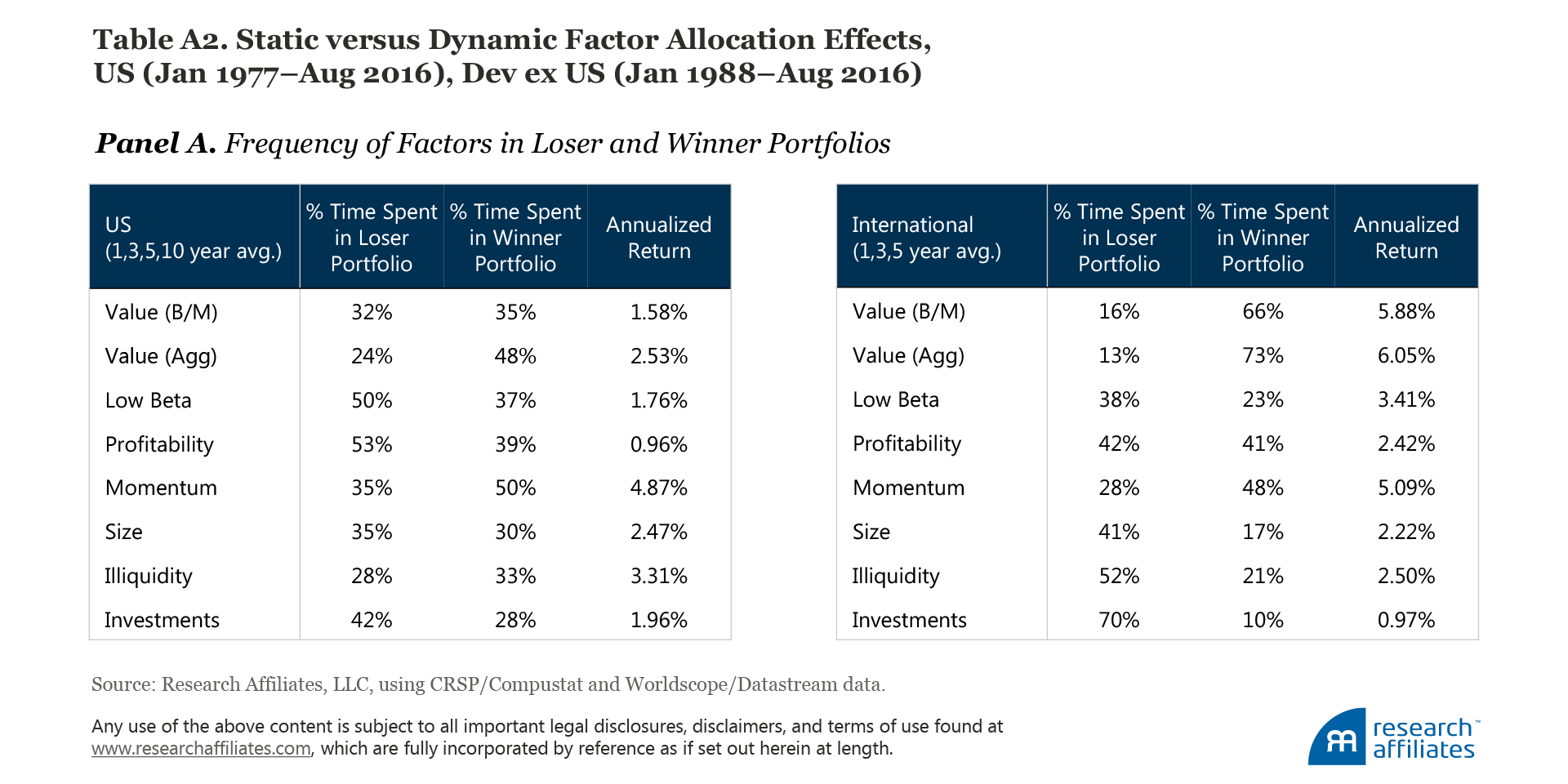
A static allocation component to the trend-chasing and contrarian factor-timing approaches merits investigation. In the US markets, where factors are usually first discovered, most spend roughly equal amounts of time in the winner and loser portfolios. Some factors, however, are not robust out of the US sample and do not work as well internationally. The trend chaser who invests in the winning factors, therefore, will tend to pick up factors such as value and momentum that work out of sample, whereas the contrarian who invests in the losing factors will tend to pick up nonrobust factors having poor international returns.
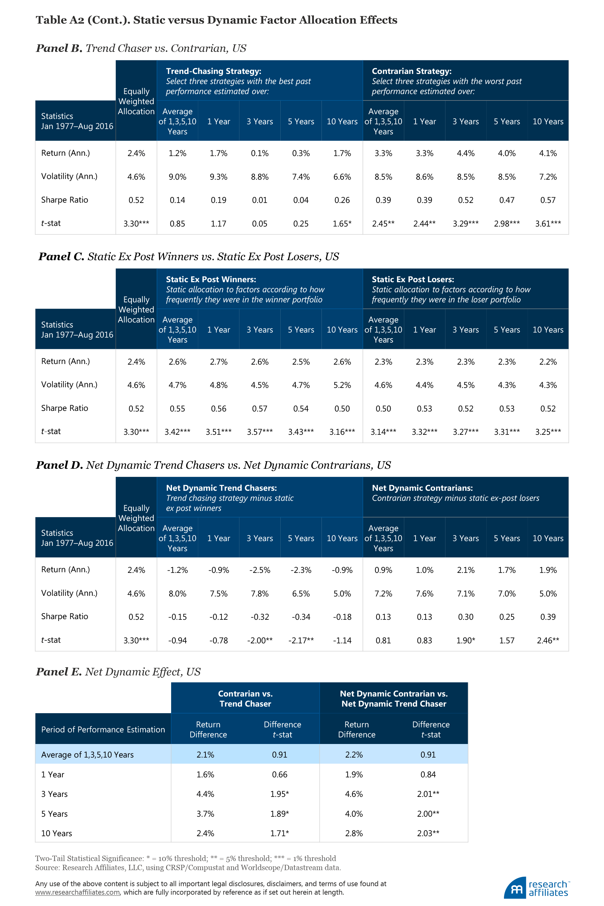
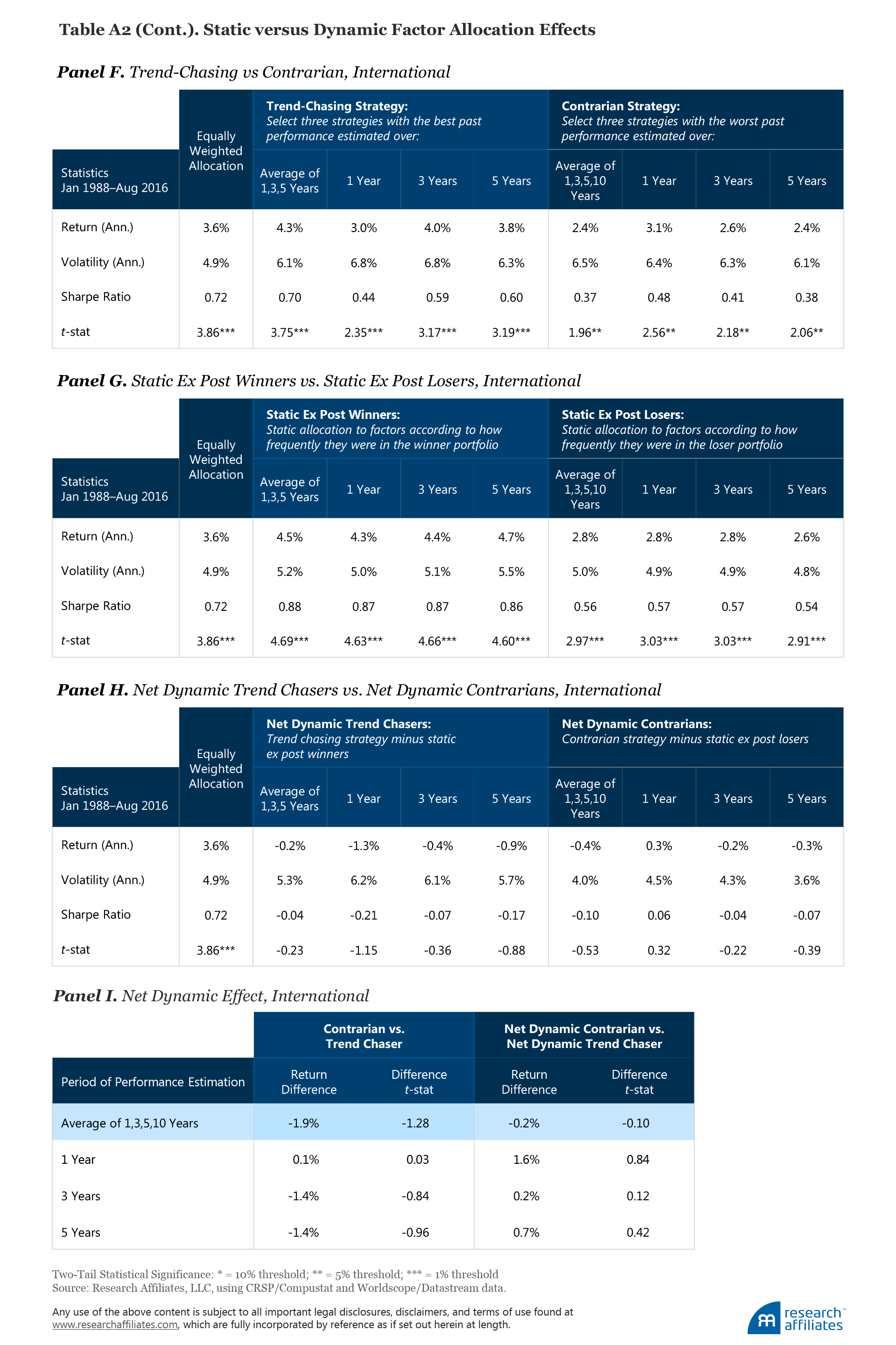
In Panels C (US) and G (International) in Table A2, we compute returns to portfolios that were given static allocations according to how frequently they appeared in the winner and loser portfolios. Subtracting these returns from those of the factor-timing trend chasers and contrarians in Panels B (US) and F (International), gives us the net effect in Panels D (US) and H (International)—the returns coming from dynamically changing factor allocations. Panels E (US) and I (International) compare the net dynamic trend chasers to the net dynamic contrarians.
By selecting recent winners, trend-chasing strategies are more likely to pick up expensive factors, but are also more likely to pick up robust factors with significant structural alpha. When we account for this tendency, we find the contrarian improves even more against the trend chaser. The ideal factor-timing strategy, therefore, would involve first evaluating which of the hundreds of factors can be expected to persist long into the future; that is, which are robust across many regions and definitions, and have sound economic or behavioral explanations for their persistence.19 Of the factors that pass these robustness checks, investors should tilt toward those that are less expensive relative to their historical valuations.
Simulation Methodology used in “Timing ‘Smart Beta’ Strategies? Of Course! Buy Low, Sell High!”
For Factors
For factor simulations in the United States we use the universe of US stocks from the CRSP/Compustat Merged Database. We define the US large-cap equity universe as stocks whose market capitalizations are greater than the median market-cap on the NYSE. For international factors (developed ex U.S.) we use the universe of stocks from the Worldscope/Datastream Merged Database. We define the international large-cap equity universe as stocks whose market-caps put them in the top 90% by cumulative market-cap within their region, where regions are defined as North America, Japan, Asia Pacific, and Europe.
The large-cap universe is then subdivided by various factor signals to construct high-characteristic and low-characteristic portfolios, following Fama and French (1993) for the US and Fama and French (2012) for international markets. (Note that slight variations in data cleaning and lagging, as well as different rebalance dates, could lead to slight differences between our factors and those of Fama and French.) As an example, in order to simulate the value factor in the United States, we construct the value stock portfolio from stocks above the 70th percentile on the NYSE by book-to-market ratio, and we construct the growth stock portfolio from stocks below the 30th percentile by the same measure. Internationally, we construct the value stock portfolio from stocks above the 70th percentile in their region (North America, Japan, Asia Pacific, and Europe) by book-to-market, and the growth stock portfolio from stocks below the 30th percentile in their region.
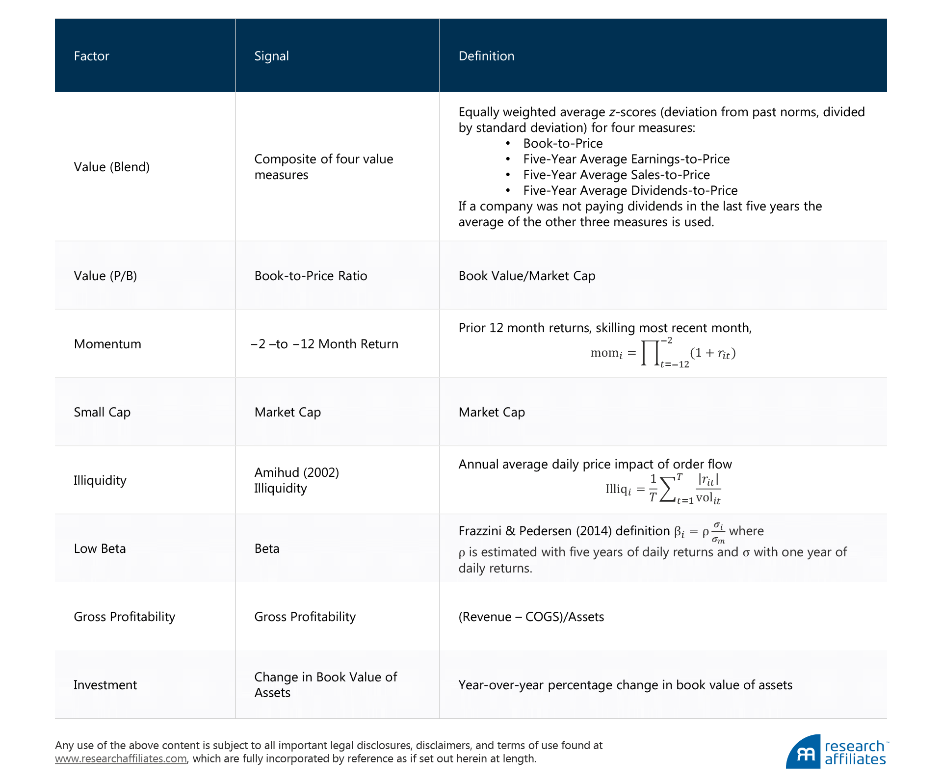
The stocks are then market-cap weighted within each of the two portfolios, which are used to form a long–short factor portfolio. Portfolios are rebalanced annually each January with the exception of momentum, which is rebalanced monthly. U.S. data extend from January 1967 to August 2016, developed ex U.S. from January 1983 to August 2016, and has been filtered to exclude ETFs and uninvestable securities such as state-owned enterprises and stocks with little to no liquidity. The signals used to sort the various factor portfolios follow:
For Smart Beta Strategies
We use the universe of stocks of the top 1,000 U.S. and developed ex U.S. companies by market capitalization for all smart betas with the exception of Fundamental Index™, for which we use the top 1,000 companies by fundamental size. The portfolios are defined as follows:
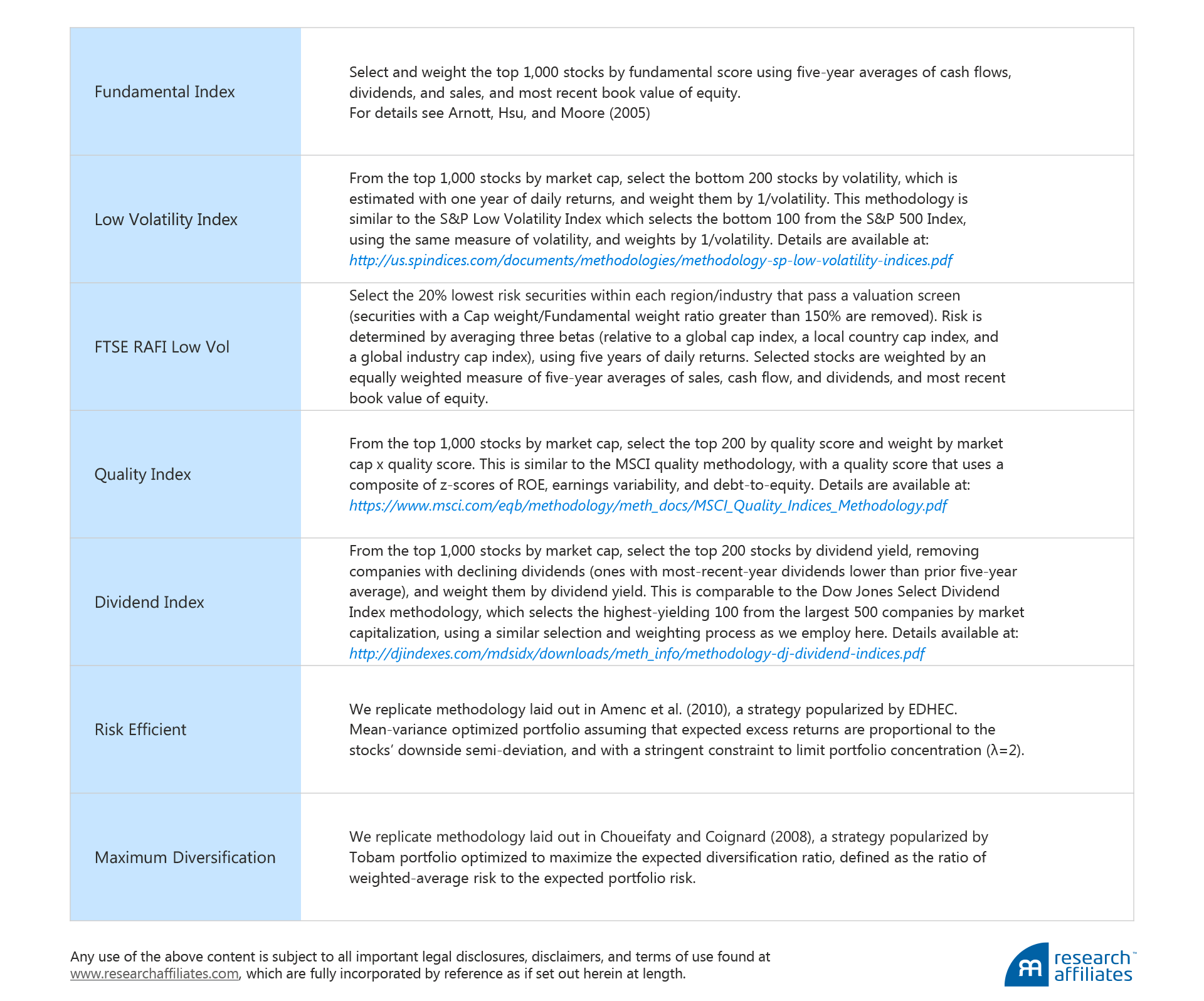
Timing Methodology
The following timing methods were employed across smart beta strategies and factors:
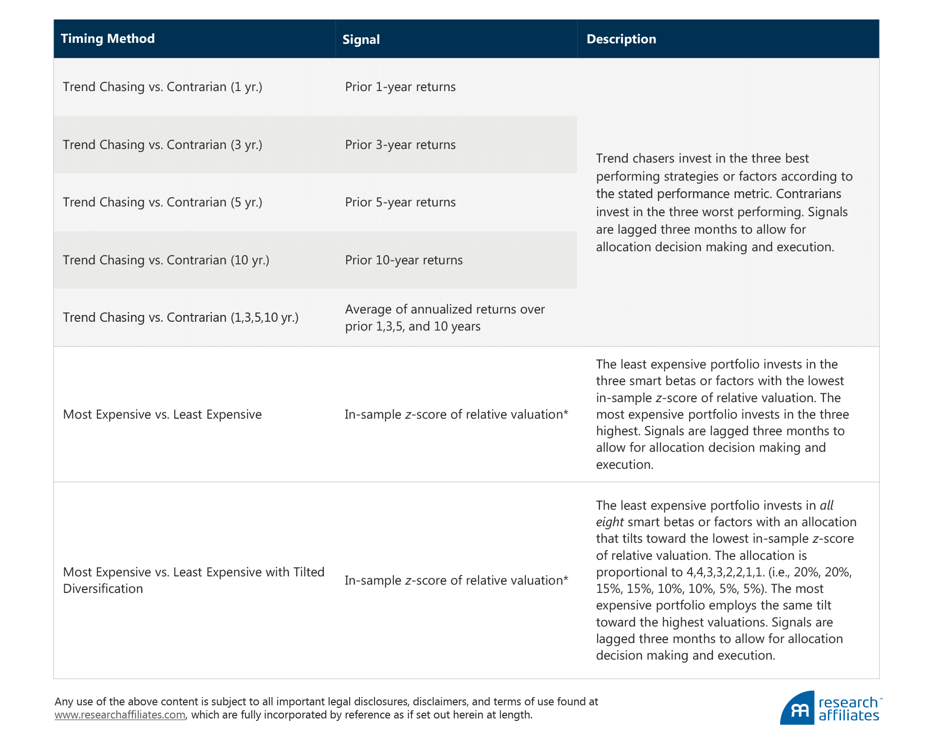
*Relative valuation is defined as an aggregate of four relative valuation measures: relative price to book (P/B), relative price to earnings (P/E), relative price to sales (P/S), and relative price to dividends (P/D). Each of these is defined as the price-to-fundamental ratio of the long side divided by the price-to-fundamental ratio of the short side in the case of factors, and the price-to-fundamental ratio of the strategy divided by the price-to-fundamental ratio of the market in the case of smart betas. For example, the relative P/B of RAFI would be 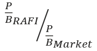 and the relative P/B of the momentum factor would be
 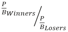 . We use five-year averages for company-level earnings, sales, and dividends in computing fundamental ratios. At the portfolio level, we then take the geometric average of relative P/B, P/E, P/S, and P/D to compute relative valuation.
Relative valuation is predictive of future factor and smart beta returns, as shown in “To Win with Smart Beta, Ask If the Price Is Right.” When comparing across strategies for the purposes exploring timing strategies, it is important to compare each portfolio’s relative valuation to its own history. We compute the in-sample z-score of relative valuation for the purposes of selecting and allocating across strategies and factors.


