Factor returns, net of changes in valuation levels, are much lower than recent performance suggests.
Value-add can be structural, and thus reliably repeatable, or situational—a product of rising valuations—likely neither sustainable nor repeatable.
Many investors are performance chasers who in pushing prices higher create valuation levels that inflate past performance, reduce potential future performance, and amplify the risk of mean reversion to historical valuation norms.
We foresee the reasonable probability of a smart beta crash as a consequence of the soaring popularity of factor-tilt strategies.
This is the first of a series on the future of smart beta.
Because active equity management has largely failed to deliver on investors’ expectations,1 investors have acquired a notable appetite for any ideas that seem likely to boost returns. In this environment, impressive past results for so-called smart beta strategies, even if only on paper, are attracting enormous inflows. Investors often choose these strategies, as they previously chose their active managers, based on recent performance. If the strong performance comes from structural alpha, terrific! If the performance is due to the strategy becoming more and more expensive relative to the market, watch out!
Performance chasing, the root cause of many investors’ travails, has three inextricably linked components. Rising valuation levels of a stock, sector, asset class, or strategy inflate past performance and create an illusion of superiority. At the same time, rising valuations reduce the future return prospects of that stock, sector, asset class, or strategy, even if the new valuation levels hold. Finally, the higher valuations create an added risk of mean reversion to historical valuation norms.
Many of the most popular new factors and strategies have succeeded solely because they have become more and more expensive. Is the financial engineering community at risk of encouraging performance chasing, under the rubric of smart beta? If so, then smart beta is, well, not very smart.
Are we being alarmist? We don’t believe so. If anything, we think it’s reasonably likely a smart beta crash will be a consequence of the soaring popularity of factor-tilt strategies. This provocative statement—especially by one of the original smart beta practitioners—requires careful documentation. In this article we examine the impact of rising valuations on many popular smart beta categories.
A Risk Premium Parable: The “New Paradigm” of 1999
A quick look back to 1999 is instructive. Over the second-half of the 20th century, the S&P 500 Index produced a 13.5% return (an annualized real return of 9.2%) and 10-year Treasuries a 5.7% return (an annualized real return of 1.6%). During this 50-year period, stocks delivered an excess return relative to bonds, let alone cash, of almost 7.5% a year!2 The investing industry embraced these historical returns as gospel in setting future return expectations—at the top of the tech bubble, pension fund discount rates and return assumptions were the highest ever, before or since, for stocks and balanced portfolios. In the late 1990s, many proclaimed a “new paradigm”: profits were no longer needed, and equity valuations could rise relentlessly. Remember “Dow 36,000”? We’re still waiting.
The problem with these forecasts is that fully 4.1% of the annualized 50-year (1950–1999) stock market return—nearly half of the real return!—came from rising valuations as the dividend yield tumbled from 8% to 1.2%. The Shiller PE ratio more than quadrupled from the post-war doldrums of 10.5x to a record 44x.3 Reciprocally, as bond yields tripled over the same period, from 1.9% to 6.6%, real bond returns were trimmed by an average 0.7% a year, creating modest capital losses atop skinny real yields. If we subtract nonrecurring capital gains (for stocks) and losses (for bonds) from market returns, the adjusted historical excess return falls to 2.5%.4,5 Thus, over this stupendous half-century for stocks, the true equity premium was 2.5%. The 7.5% gap between stocks and bonds was an unsustainable change in relative values!
The lofty past returns not only laid a foundation for lofty expectations, but also led to valuations that virtually guaranteed far lower future returns. As noted by Arnott and Bernstein (2002), investors in 1999 should not only have adjusted past returns to remove the impact of rising valuation levels, they should also have adjusted expectations to reflect the lowest-ever stock market yields and the above-average real bond yields.6 Investors could even have gone further, adjusting expectations to reflect the substantial likelihood of mean reversion. The higher equity valuations of today continue to translate into lower future returns than most investors expect.
Nowadays, astute observers increasingly “get it,” at least to the point of subtracting valuation gains from past returns. A 2015 survey of investment consultant return expectations produced an average forward “long-term” (10-year) U.S. nominal equity return of 6.8% a year;7 at the start of the century, return expectations over a similar horizon were in the double digits.8,9 After 15 years and two punishing bear markets, investors are figuring out past returns need to be adjusted for the sometimes large impact of rising valuations, and expected returns need to be adjusted for the sometimes large impact of mean reversion. Even after the stellar bull market since early 2009, the annualized real return on U.S. stocks from 2000 to 2015 has averaged a scant 1.9% (not even matching the average dividend yield), while U.S. bonds have delivered an outsized real return of 3.6%. The “excess return” for stocks has been negative by a daunting 1.7% a year.
Our parable holds a relevant lesson for smart beta investors: a lengthy return history, even 50 years, does not guarantee a correct conclusion. Investors need to look under the hood to understand how a strategy or factor produced its alpha. We compare several popular strategies’ current valuations relative to history, and find that for many, much of the historical value-add—in some cases, all!—has come primarily from the “alpha mirage” of rising valuations.
Academia is no less prone than the practitioner community to be a slave to past returns. Anomalies and factor returns tend to appear and then fade, depending on recent performance. Of course, no one will bother to publish a factor or a strategy that fails to add value historically; this encourages data mining and selection bias. In recent years, several hundred “factors” have been published, most showing statistically significant “alpha” and a path to higher future returns.10
Value-add can be structural (hence, plausibly a source of future alpha) or situational (a consequence of rising enthusiasm for, and valuation of, the selected factor or strategy). Few, if any, of the research papers in support of newly identified factors make any effort to determine whether rising valuations contributed to the lofty historical returns. The unsurprising reality is that many of the new factors deliver alpha only because they’ve grown more expensive—absent rising relative valuations, there’s nothing left!
The Impact of Valuations on Returns: The Value Factor
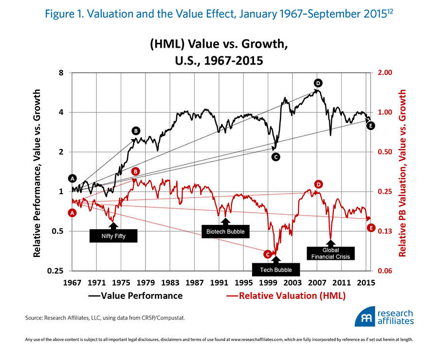
The value effect was first identified in the late 1970s, notably by Basu (1977), in the aftermath of the Nifty Fifty bubble, a period when value stocks were becoming increasingly expensive, priced at an ever-skinnier discount relative to growth stocks. More recently, for the past eight years, value investing has been a disaster with the Russell 1000 Value Index underperforming the S&P 500 by 1.6% a year, and the Fama–French value factor in large-cap stocks returning −4.8% annually over the same period. But, the value effect is far from dead! In fact, it’s in its cheapest decile in history. In Figure 1 we compare the performance of the classic Fama–French value factor11 (black line) with changes in its relative price-to-book (P/B) valuation levels (red line) from January 1967 to September 2015. When the black line is rising, value stocks are becoming more richly priced (i.e., the market is paying a shrinking premium for growth) and value is outperforming. Conversely, when the black line is falling, value stocks are almost always getting cheaper (i.e., the market is paying up for growth stocks) and value is underperforming. (Click Here for a full description of the simulation methodology.)
The red line shows the relative P/B valuation level (the average P/B ratio for the value portfolio divided by the average P/B ratio for the growth portfolio) as it changes over time. Because value always trades cheaper than growth—by its very definition—the valuation ratio, shown on the right scale, often is far lower than 1.0. When the red line is rising, value is winning (i.e., getting more richly priced than it was before, relative to growth), and when the red line is falling, growth is winning (i.e., getting more expensive, relative to value). Not surprisingly the black and red lines move up and down together. The lines diverge, however, which means value has historically had a structural alpha, not wholly reliant on becoming more expensive.
How many practitioners who rely on the value factor take the time to gauge whether the factor is expensive or cheap relative to historical norms? If they took the time to do so today, they would find value is currently cheaper than at any time other than the height of the Nifty Fifty13 (1972–73), the tech bubble (1998–2003), and the global financial crisis (2008–09).
Relative Valuation Levels in the “Factor Zoo”
Relative valuation affects factor returns throughout the factor zoo.14 We find that the efficacy of a factor-based strategy or a factor tilt (included by many under the smart beta umbrella) is strongly linked to changes in relative valuation, that is, whether the strategy is in vogue (becoming more richly priced) or out of favor (becoming cheaper).
How do most investors assess whether these factors and strategies work? The same way they figure out the effectiveness of conventional active managers: past performance! How do academics determine which factors can get them published? Again, past performance! What do most investors and academics miss? The effects of changing relative valuation levels, of course!
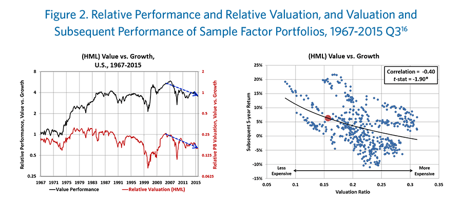
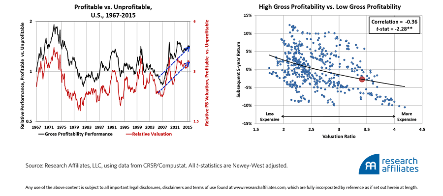
Relative Valuation in Factor Portfolios. We begin our analysis by examining the relative performance and relative valuations for six sample factor portfolios: value, positive momentum, small cap, illiquid, low beta, and high gross profitability. As illustrated in Figure 2, performance appears closely matched to changes in relative valuation levels for four of the six factors, with the exception of momentum and perhaps low beta (as in Figure 1, the black line tracks factor performance and the red line tracks P/B valuation level for the long sides of the portfolios relative to the short sides). Momentum and low beta share the characteristic of rapid turnover, which means that the changes in valuation will change with portfolio changes, rather than from the stocks becoming more or less expensive, relative to the market. The momentum of a stock has essentially no correlation from one year to the next; beta has a substantial estimation error, and thus can change rapidly for both legitimate and spurious reasons.15
The positive momentum factor portfolio will usually trade at a premium because high momentum stocks have, by definition, risen in price. On rare occasions, when deep value stocks have turned sharply and are exhibiting positive momentum, the high momentum portfolio might even trade more cheaply than the low momentum portfolio. When stocks with positive momentum are cheaper relative to the market than their historical norms, the mere act of fading momentum can drive an individual stock out of the positive momentum portfolio before it enjoys any mean reversion in valuation. A lesson we can draw from this is the higher a strategy’s turnover, the less informative are valuation changes in understanding the strategy’s performance and predicting its future performance.
A second lesson we take from our analysis is that as the market evolves, the “normal” valuation level for a strategy may change. A good example is provided by low beta investing, a factor only recently gaining popularity, and the only one of the six we analyze lacking a statistically significant relationship. Although the strategy offers a market-like return with lower risk, it has high tracking error risk vis-à-vis the market. The virtually guaranteed result is prolonged periods of substantial underperformance, especially as in the near-continuous bull market of the 1990s.17 Over the last 15 years, however, two bear markets and the accompanying muted cumulative returns have forced investors to reconsider. Large asset flows into low beta products are now driving valuation levels far above their historical norms. Low beta’s end-point in relative valuation is near an all-time peak, meaning the historical link between relative valuation levels and returns will seem weak, even if it’s not (since these recent high valuations have not yet had the chance to mean revert).
The scatterplots in Figure 2 compare relative valuation and subsequent relative performance for each of the factor portfolios. This relationship is the flip side of the relative and valuation-adjusted performance relationship. If a strong link exists between relative valuation and cumulative relative performance (graphs figure-left), the market’s chasing of or fleeing from stocks with a particular factor exposure creates much of the factor’s return. The same run-up in relative valuation that boosts past relative performance—the typical driver of asset management choices—just as assuredly sets the stage for subsequent lower returns as a consequence of mean reversion. The statistical significance of most of the factors confirms the effect is real—so much for the random walk!
The red dot in the scatterplots indicates the current valuation level of each factor. We will review current valuation levels—making some interesting and surprising revelations—in a later article. In the meantime, this peek into current valuations shows that some of the most popular factors are trading at expensive relative valuations compared with their own historical norms.
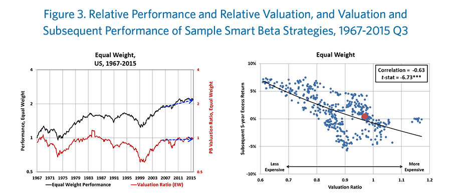
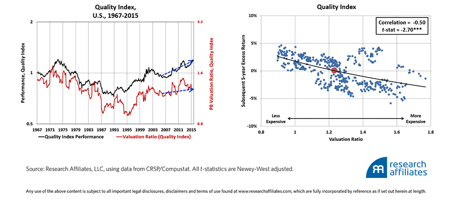
Relative Valuation in Smart Beta Portfolios. We examine six smart beta portfolios to determine if they exhibit the same pattern. Most of the six conform to our definition of smart beta, which is much narrower than the market’s. We subscribe to a core definition—the strategy must sever the link between the price of a stock and its weight in the portfolio—and a weaker requirement: a smart beta strategy should include most of the advantages of conventional indexing, such as low turnover, broad market representation, liquidity, capacity, transparency, ease of testing, low fees, and so forth (Arnott and Kose, 2014). Our analysis, described in Figure 3, includes six strategies: equal weight (the 1,000 largest-cap stocks, equally weighted), Fundamental Index™, risk efficient (popularized by EDHEC), maximum diversification (popularized by TOBAM), low volatility (based on the S&P methodology), and quality (based on the MSCI Quality Index methodology, which uses profitability, leverage, and earnings volatility as a definition of quality).18 Of these, only the quality strategy anchors on cap weighting and would not qualify as smart beta under our narrow definition. For each, we use the published methodology, reconstituting and reweighting annually at year-end in a universe of the 1,000 largest market-cap stocks.19 (Click Here for a full description of the simulation methodology.)
Just like in the factor zoo, the cumulative performance of each smart beta strategy largely co-moves with changes in valuation. We can make several important observations. For equal weight and Fundamental Index, a significant wedge between performance and relative valuation level develops over time. For the maximum diversification and risk efficient strategies, the return due to changes in valuation is significantly more volatile than for the other strategies. The volatility is being driven by substantial changes in portfolio composition. As a result, changes in valuation will be a less informative metric for these two strategies than for others; further supporting this explanation is the low correlation (−0.15) of maximum diversification’s valuation level with its subsequent performance. Low volatility’s story is similar to the one told by the low beta factor: changing valuations explain much of the past performance. Quality weaves an interesting tale as well. Performance was less than impressive over the years 1973 to 1990 as valuations started the period quite high, but improved markedly as valuations bottomed out in the early 1990s and began to climb.
The scatterplots in Figure 3 show, quite in the spirit of Arnott and Bernstein (2002), that the valuation levels for smart betas are as informative of future performance for the strategies as they are for the markets in general. As noted earlier, we will review current valuations (red dot in figure scatterplots) in a later article, but this quick preview suggests many smart beta strategies and factors are more expensive than historical norms. We should beware the alpha mirage inherent in mean-reverting valuations!
Valuation-Adjusted Performance: A Cautionary Tale. Let’s compare the excess returns of the six factor-tilt strategies and the six smart beta strategies. We look at the latest 10 years (2005 Q3–2015 Q3) and almost 49 years (1967–2015 Q3). Many investors believe 10 years is long enough to assess a strategy’s ability to deliver future performance. After all, active manager track records are often considered relevant after just 5 years. Some even argue recent performance—the past 10 or 20 years—is most representative of future performance because markets are very different today compared to generations past. We strenuously disagree. Our parable, “The New Paradigm of 1999,” demonstrates even a half-century (two generations!) is not necessarily long enough to draw the correct conclusions.
To improve outcomes, investors should seek more data, ideally covering a wide range of market environments, fads, and shifting investor preferences. Sadly, commercial options are not helpful in this regard. A quick survey of two of the larger factor index providers shows average factor indices have track records between 14 and 17 years.20 One substitute for “more data” is to at least subtract the return that comes from changes in relative valuation, so investors won’t fall prey to the seduction of performance chasing and don’t mistake a relative-performance bull market (in a stock, style, factor, sector, asset class, or strategy) for alpha.21
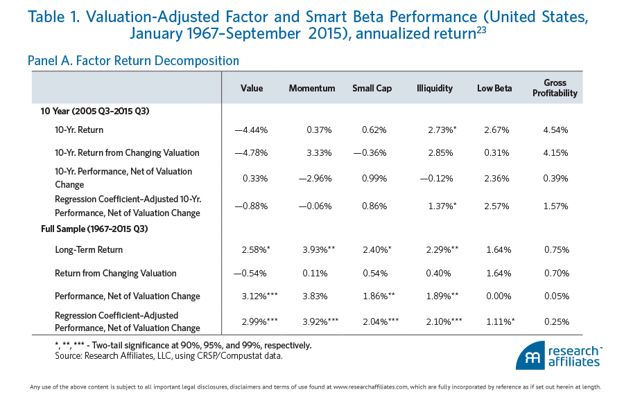
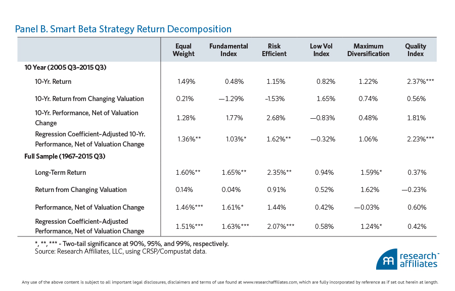
In Table 1 we report the return decomposition for each factor and smart beta strategy, showing how much of the performance comes from changes in valuation. We provide two estimates of valuation-adjusted performance: 1) performance net of valuation change, which is a simple difference between return and the concurrent change in valuation; and 2) adjusted performance net of valuation change, a more conservative estimate, which we calculate by subtracting only a regression-based fraction of the changes in valuation.22
Over the last 10 years, of the six factors, gross profitability (the quality definition most popular in current academic research) had the best performance, while value had the worst. We also find that essentially all of the outperformance for profitability is due to rising valuations. When we subtract the returns associated with the rising popularity, and therefore rising relative valuation, of high-profit companies versus low-profit companies, the gross profitability factor loses more than 90% of its historical efficacy, delivering 10-year performance net of valuation change of just 0.39%. The more conservative regression-based performance estimate trims excess return by two-thirds, from 4.54% to a much less spectacular 1.57%.
Rising valuations also provided a substantial tailwind for momentum and illiquidity over the last decade. This means gross profitability, momentum, and illiquidity are all considerably more expensive today than they were 10 years ago. Over this same period, we see value has floundered because it was out of favor and becoming ever cheaper!
A look at the full-sample period shows, first, that all of the factors had positive performance. This should not be surprising as the popular factors were identified and published because they had high past performance. Factors and strategies with marginal or insignificant long-term performance will routinely be discarded. Second, the two factors with the lowest overall full-sample performance are gross profitability and low beta, despite their brilliant performance record during the past decade.
Even over nearly a half-century, a shocking portion of the return for several factors comes from rising relative-valuation levels. Net of rising valuation, the value added by low beta disappears entirely or is reduced by a third, considering the more conservative regression-adjusted estimate; the same holds true for gross profitability. Should investors really expect to be rewarded for profitability or quality? Shouldn’t we accept a lower return for safer assets? Some of the strategies, for example, low beta, may still be an attractive investment, but for their risk-reducing characteristics not for the alpha they have historically provided, net of their rising popularity and relative valuation. These data suggest that common sense prevails: lower risk, higher quality, and safety have all earned a strong premium only as a consequence of becoming more expensive! Will this upward adjustment in relative valuation prove permanent? Figure 2 suggests otherwise. But even if it is, we cannot rely on rising valuations to continue to create an illusion of alpha.24
The six smart beta strategies all delivered positive excess returns over both the 10-year period and the full-sample period. But, net of the effect of changing valuations, results are mixed. The strategies hurt most by the declining valuations over the last decade are risk efficient and Fundamental Index. But despite valuations moving in an adverse direction, both strategies were able to outperform in the last 10-year period.25
The low vol, maximum diversification, and quality strategies all experienced a large performance tailwind from rising relative valuations. Over the last decade, the low vol strategy, for example, delivered 0.82% a year in return. Because the strategy became significantly more expensive over the period, the return from changing valuations was 1.65% a year. Thus, more than 100% of its return came from expanding valuations! Over the full-sample period, maximum diversification generated performance of 1.59% a year; without the 1.62% a year it earned from rising valuations, performance would have been negative. Our analysis of past performance accompanied by rising valuations does not make a very convincing case that similar performance can be repeated in the future.
In the last decade, quality generated the best performance of all smart betas at 2.37% a year, helped by rising valuations. This result is a backtest, and the best way to validate a backtest is to use out-of-sample data. During the 39-year period 1967–2005, quality delivered a −0.14% annualized return. Not surprisingly, in the longer 49-year sample, quality had the worst performance of all smart betas at 0.37% a year. Interestingly, unlike the gross profitability factor for which close to 100% of both 10-year and full-sample returns is attributable to rising valuations, the 0.37% a year return for the quality factor did not come from rising valuations. This highlights another problem with quality investing: quality portfolios can be quite sensitive to the definition being used. A portfolio formed on gross profitability can be very different from a portfolio formed on quality, which is based on profitability, leverage, and earnings volatility.
Conclusion
Arnott and Bernstein (2002, p. 64) observe that “the investment management industry thrives on the expedient of forecasting the future by extrapolating the past.” But, we must make every effort to avoid being duped by historical returns. We can accomplish this by netting out the effect of changing valuations on past returns, which arguably gives us a more reliable historical “normal” expected return. Then, we need to go one step further. We should also adjust our expectations to allow for the possibility of mean reversion to historical norms for relative valuation.
The steady backtests rolling out of smart beta proliferators indicate a 2–3% excess return can be earned from a variety of “alpha sources.” Normal returns are being extrapolated based solely on past performance, not at the equity asset class level but within it. But this reassuring message has two primary and interrelated flaws.
First, many of these alpha claims are based on a 10- to 15-year backtest that won’t cover more than a couple of market cycles. Second, such a short time span is very vulnerable to distortion from changing valuations. Our analysis shows that valuation has been a large driver of smart beta returns over the short and even long term. How much can we reasonably expect in future returns from these factors and strategies, net of valuation change? For some strategies perhaps a great deal, and for others, not much.
Today, only the value category shows some degree of relative cheapness, precisely because its recent performance has been weak! Generally speaking, normal factor returns, net of changes in valuation levels, are much lower than recent returns suggest. Investors entering the space should adjust their expectations accordingly.
Academe would do well to explore how much of the success of their favorite factors (and the dozens of new factors published each year) is coming from rising relative valuation levels. If rising valuation levels account for most of a factor’s historical excess return, that excess return may not be sustainable in the future; indeed our evidence suggests that mean reversion could wreak havoc in the world of smart beta. Many practitioners and their clients will not feel particularly “smart” if this forecast comes to pass.
In the next two articles of this series, we will discuss which factor-tilt and smart beta strategies are over- or undervalued relative to historical norms. Some may be priced to deliver negative future alpha, not positive! And we will objectively test the comparative efficacy of performance chasing in the factor zoo (i.e., favoring the factor tilts and smart beta strategies with the best recent performance) against investing in strategies with abnormally poor recent performance. The results are eye-opening to say the least.
Endnotes
1. Active managers have failed to deliver on clients’ return expectations through no fault of their own. This result is almost a tautology. When the capitalization-weighted index strategies are removed from the cap-weighted market, we’re left with more or less the same portfolio, that is, the holdings of active managers and individual investors. Collectively, because of trading costs and management fees, active managers and individual investors cannot beat the market; most will underperform. Certainly, some active managers will win. In fact, Berk and Green (2004) estimate that before fees about 80% of active managers do win, chiefly at the expense of individual investors. Unfortunately, even if active managers do win, Malkiel (2005) estimates that, on average, fees and other expenses consume most of the outperformance, leaving an average investor in active funds slightly worse off than if they had invested in a low-fee passive alternative. Collectively, an active manager’s very important role is to increase market efficiency by identifying mispricing. If investors collectively chose only passive investing, markets would be extremely inefficient both in terms of investment outcomes and aggregate capital allocation. French (2008) estimates investors collectively pay 67 bps in market value annually for this price discovery, a remarkably reasonable societal cost for the efficient allocation of capital in the aggregate economy.
2. Many investors erroneously label this return difference a risk premium. This is a dangerous and expensive mistake. A risk premium is a forward-looking expectation; excess return is a backward-looking historical return difference. Past excess returns and the expected risk premium are not the same thing.
3. The Shiller Price/Earnings (PE) ratio, also known as the cyclically adjusted PE (CAPE), is simply the real level of a market index (or individual stock) divided by the previous 10-year average of real earnings. This simple adjustment assures that our measure of market valuation is not distorted by current peak or trough earnings.
4. Over the 1950–1999 period, if 4.1% of the 9.2% real return for stocks came from rising valuation multiples, then absent that rise in valuation multiples, the real return would have been 4.9% (9.2% minus 4.1% minus 0.2% from the compounding effect). Net of the capital losses associated with rising bond yields, the average real bond return for the same period would have been 2.3% (1.6% plus 0.7%). Subtracting the 2.3% bond return from the 4.9% stock return, and adjusting the difference for compounding, the adjusted historical equity excess return is 2.5%.
5. The market valuation levels cited are as of December 1999.
6. Arnott and Ryan (2000, 2001) argued the risk premium was dead, a position widely dismissed at the time as utterly implausible. What’s been the excess return for U.S. stocks relative to bonds since then, despite current nosebleed valuation levels? Less than zero! Arnott and Ryan readily acknowledged that, with a large enough shift in relative valuation between stocks and bonds, the risk premium could—like the phoenix—come back from the dead, reviving the positive risk premium that finance theory and common sense suggest should prevail.
7. “Survey of Capital Market Assumptions: 2015 Edition,” Horizon Actuarial Services, LLC, July 2015.
8. The Duke CFO Global Business Outlook, a quarterly survey of chief financial officers of public and private companies around the globe, showed an average 10-year nominal equity return forecast of 6.5% as of December 2015. The same survey conducted in June 2000 showed an average 10-year nominal return forecast of 10.5%. Although CFOs are not money managers or consultants, they are usually aware of standard valuation techniques and use them to explain their company’s share performance relative to the market.
9. It is encouraging to see more realistic expectations, but the fact that valuations can detract, sometimes sizably, from long-term equity returns should not be ignored. For a fuller explanation, see Brightman, Masturzo, and Beck (2015).
10. The problems of data mining and identifying spurious factors have attracted a lot of attention recently in both the academic and practitioner communities. Harvey, Liu, and Zhu (2015) and Harvey and Liu (2015) propose a multiple-testing framework to adjust t-statistics as a means of reducing the number of spurious factors that need to be considered. Hsu, Kalesnik, and Viswanathan (2015) propose a practitioner-oriented procedure to identify more robust factors by perturbing factor definitions, examining factor robustness across geographies, and incorporating transaction costs into estimates of excess returns.
11. The performance line (in black) tracks the cumulative return of the Fama–French value, or high-minus-low (HML), factor for large-cap stocks. The factor return series is computed by taking the monthly difference between the return of a cap-weighted portfolio of the 30% of large-cap stocks trading at the highest book-to-price (B/P) ratio (value stocks) versus a cap-weighted portfolio of the 30% of large-cap stocks trading at the lowest B/P ratio (growth stocks). The portfolios are constructed once a year and are not subject to monthly reconstitution or rebalancing.
12. Relative valuation is defined for factors as  and for smart beta strategies as
13. The Nifty Fifty refers to 50 NYSE stocks—including stocks such as Xerox, IBM, Polaroid, Mattel, Avon, and Coca-Cola—proclaimed in the 1960s and 1970s to be so dominant in their industry and so reliable in their growth that they were deemed to be good investments at any valuation.
14. Cochrane (2011) first coined the term “zoo of new factors.” Jason Hsu appropriated and abbreviated this to factor zoo.
15. All of the results presented in this article ignore transaction costs. Investors interested in practically implementing these strategies should adjust excess return estimates for the trading costs associated with them. Novy-Marx and Velikov (2014) and Hsu et al. (forthcoming) estimate trading costs for the more common factors and find many associated with intensive trading, such as momentum, do not exhibit excess return after being adjusted for trading costs under an assumption of index-like implementation. To benefit from many of these factors, investors need access to index funds that can materially reduce transaction costs and access to fund managers who can materially reduce transaction costs through careful execution.
16. The importance of current valuations in predicting future value strategy returns was first independently demonstrated by Asness et al. (2000) and Cohen, Polk, and Vuolteenaho (2001). Li and Lawton (2014) and Garcia-Feijóo et al. (2015) demonstrated that valuations are extremely important for low beta/low volatility strategies.
17. In the 1990s, low beta stocks (i.e., the long side of the low beta factor portfolios in our study) posted an average return of 10.0%, underperforming high beta stocks (i.e., the high beta side of the same factor portfolio) by 12.5% over the same period and underperforming S&P 500 by 8.2% annually.
18. We use the methodology of Arnott, Hsu, and Moore (2005) to replicate the Fundamental Index strategy; the methodology of Amenc et al. (2010) to replicate the risk efficient strategy; and the methodology of Choueifaty and Coignard (2008) to replicate the maximum diversification strategy. We rely on the following for low volatility and quality, respectively: S&P Low Volatility Index Methodology and MSCI Quality Indices Methodology.
19. For the Fundamental Index strategy, the selection of the universe is as important as the portfolio weighting method. In our analysis the universe is the 1,000 largest companies, weighted on four fundamental measures of company size: most recent year-end book value and the five-year average of sales, cash flow, and dividends paid. The average of these four measures of company size—not per share, and not looking at the valuation ratios—is the basis for identifying the 1,000 largest businesses and for their weights in the portfolio.
20. We surveyed all MSCI and Russell factor index strategies. As of December 2014, the average index history length was 16.4 years for MSCI and 13.7 for Russell. The average across both index providers was 15.1 years.
21. A popular Wall Street aphorism, is “never mistake a bull market for genius.” This is every bit as applicable in assessing smart beta strategies and factors as it is for assessing manager or market performance.
22. We compute the regression coefficient–adjusted return by regressing factor or smart beta excess returns on a rolling 12-month basis against the concurrent change in relative valuations (i.e., the movement in price to book, relative to the market, over the same span). If done for a randomly constructed market-like portfolio, the beta would be 1.0: if the portfolio beat the market by 10%, it presumably got 10% richer in relative valuation, and vice versa. Because the portfolios are rebalanced and reconstituted annually (or in the case of momentum, monthly), the linkage weakens.
23. We use the following return decomposition to compute the return from a change in valuation:

from which we derive  to define the return from a change in valuation. The difference between the return and the return due to a change in valuation is the valuation-adjusted return.
24. Optimists might expect another upward adjustment in valuation of the same level, much like the optimists of the late 1990s extrapolated equity returns, tacitly forecasting ever-higher Shiller PEs.
25. We note that both of these strategies, on average, have significant positive value exposure according to Arnott et al. (2013). Some claim that the Fundamental Index strategy is just a repackaged value strategy. But, how did these strategies manage to outperform over a period when the value factor did so poorly? We conjecture that part of the difference comes from dynamic value exposure: if a strategy has relatively little value exposure when value is expensive, and a lot of value exposure when value is cheap, such a strategy can still have positive performance despite value doing poorly over the period.
References
Amenc, Noël, Lionel Martellini, Jean-Christophe Meyfredi, and Volker Ziemann. 2010. “Passive Hedge Fund Replication: Beyond the Linear Case.” European Financial Management, vol. 16, no. 2 (March):191–210.
Amihud, Yakov. 2002. “Illiquidity and Stock Returns: Cross-Section and Time-Series Effects.” Journal of Financial Markets, vol. 5, no. 2:31–56.
Arnott, Robert D., and Peter L. Bernstein. 2002. “What Risk Premium Is ‘Normal’?” Financial Analysts Journal, vol. 58, no. 2 (March/April):64–85.
Arnott, Robert D., Jason Hsu, Vitali Kalesnik, and Phil Tindall. 2013. “The Surprising Alpha from Malkiel’s Monkey and Upside-Down Strategies.” Journal of Portfolio Management, vol. 39, no. 4 (Summer):91–105.
Arnott, Robert D., Jason Hsu, and Philip Moore. 2005. “Fundamental Indexation.” Financial Analysts Journal, vol. 61, no. 2 (March/April):83–99.
Arnott, Robert D., and Engin Kose. 2014. “What ‘Smart Beta’ Means to Us.” Research Affiliates Fundamentals (August).
Arnott, Robert D., and Ronald Ryan. 2000. “The Death of the Risk Premium: Consequences of the 1990s.” Investment Management Reflections, No. 1, First Quadrant.
———. 2001. “The Death of the Risk Premium: Consequences of the 1900s.” Journal of Portfolio Management, vol. 27, no. 3 (Spring):61–74.
Asness, Clifford S., Jacques A. Friedman, Robert J. Krail, and John M. Liew. 2000. “Style Timing: Value versus Growth.” Journal of Portfolio Management, vol. 26, no. 3 (Spring):50–60.
Basu, Sanjoy. 1977. “Investment Performance of Common Stocks in Relation to Their Price-Earnings Ratios: A Test of the Efficient Market Hypothesis.” Journal of Finance, vol. 32, no. 3 (June):663–682.
Berk, Jonathan B., and Richard C. Green. 2004. “Mutual Fund Flows and Performance in Rational Markets.” Journal of Political Economy, vol. 112, no. 6 (December):1269–1295.
Brightman, Chris, Jim Masturzo, and Noah Beck. 2015. “Are Stocks Overvalued? A Survey of Equity Valuation Models.” Research Affiliates Fundamentals (July).
Choueifaty, Yves, and Yves Coignard. 2008. “Toward Maximum Diversification.” Journal of Portfolio Management, vol. 35, no. 1 (Fall):40–51.
Cochrane, John. 2011. “Presidential Address: Discount Rates.” American Finance Association, July 19.
Cohen, Randolph B., Christopher Polk, and Tuomo Vuolteenaho. 2001. “The Value Spread.” NBER Working Paper 8242.
Fama, Eugene, and Kenneth French. 1993. “Common Risk Factors in the Returns on Stocks and Bonds.” Journal of Financial Economics, vol. 33, no. 1:3–56.
Frazzini, Andrea, and Lasse H. Pedersen. 2014. “Betting Against Beta.” Journal of Financial Economics, vol. 111, no. 1 (January):1–25.
French, Kenneth R. 2008. “Presidential Address: The Cost of Active Investing.” American Finance Association, July 19.
Garcia-Feijóo, Luis, Lawrence Kochard, Rodney N. Sullivan, and Peng Wang. 2015. “Low-Volatility Cycles: The Influence of Valuation and Momentum on Low-Volatility Portfolios.” Financial Analysts Journal, vol. 71, no. 3 (May/June):47–60.
Harvey, Campbell R., and Yan Liu. 2015. “Lucky Factors.” (December 21). Available on SSRN.
Harvey, Campbell R., Yan Liu, and Heqing Zhu. 2015. “…and the Cross-Section of Expected Returns.” (February 3). Available on SSRN.
Hsu, Jason, Vitali Kalesnik, Noah Beck, and Helge Kostka. Forthcoming. “Will Your Factor Deliver? An Examination of Factor Robustness and Implementation Costs.”
Li, Feifei, and Philip Lawton. 2014. “True Grit: The Durable Low Volatility Effect.” Research Affiliates Fundamentals (September).
Malkiel, Burton G. 2005. “Reflections on the Efficient Market Hypothesis: 30 Years Later.” Financial Review, vol. 40, no. 1 (February):1–9.
Novy-Marx, Robert, and Mihail Velikov. 2014. “A Taxonomy of Anomalies and Their Trading Costs.” NBER Working Paper No.w20721 (December). Available at SSRN.
Simulation Methodology Used in “How Can ‘Smart Beta’ Go Horribly Wrong?”
For Factors
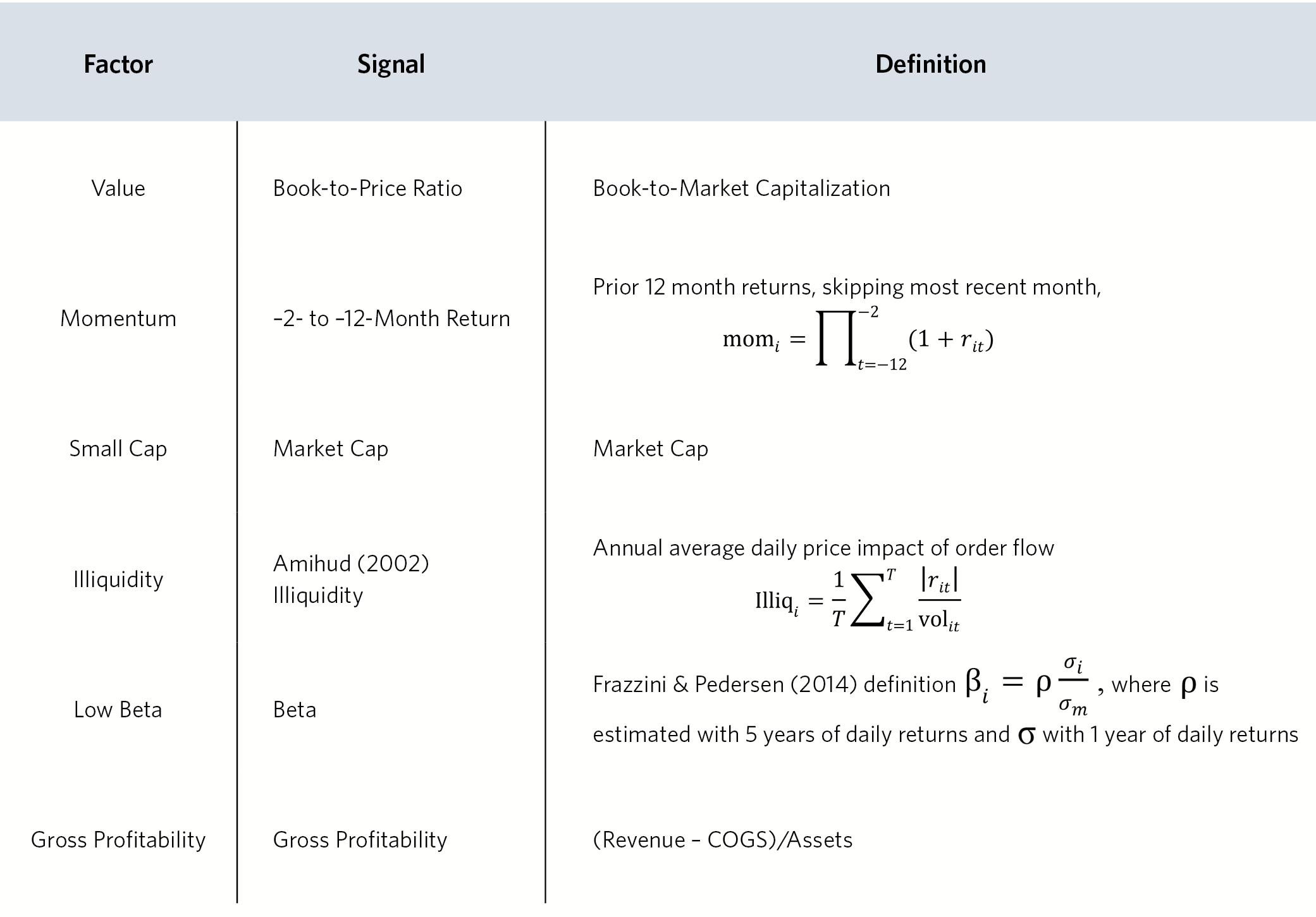
For factor simulations we use the universe of U.S. stocks from the CRSP/Compustat Merged Database. We define the U.S. large-cap equity universe as stocks whose market capitalizations are greater than the median market cap on the NYSE. The large-cap universe is then subdivided by various factor signals to construct high-characteristic and low-characteristic portfolios, following Fama and French (1993) (Note that slight variations in data cleaning and lagging, as well as different rebalance dates, could lead to slight differences between our factors and those of Fama and French). As an example, in order to simulate the value factor, we construct the value stock portfolio from stocks above the 70th percentile on the NYSE by book-to-market ratio, and we construct the growth stock portfolio from stocks below the 30th percentile by the same measure. The stocks are then market-cap weighted within each of the two portfolios, which are used to form a long/short factor portfolio. Portfolios are rebalanced annually each January with the exception of momentum, which is rebalanced monthly. U.S. data extend from 1967 to 2015 Q3. The signals used to sort the various factor portfolios follow:
For Smart Betas
We use the universe of stocks of the top 1,000 U.S. companies by market capitalization for all smart betas with the exception of Fundamental Index™, for which we use the top 1,000 companies by fundamental size.
Equal Weight
We select the top 1,000 companies by market capitalization and equally weight them.
Fundamental Index
We select and weight the top 1,000 companies by composite fundamental score using five-year averages of cash flows, dividends, and sales, and most recent book value of equity. Details are available in Arnott, Hsu, and Moore (2005).
Risk Efficient
We construct a mean-variance-optimized portfolio, assuming that the expected excess return of a stock is proportional to its downside semi-deviation, and imposing a stringent constraint to limit portfolio concentration (λ = 2). Details are available in Amenc et al. (2010).
Low Volatility Index
We select the bottom 200 stocks by volatility within the universe of the top 1,000 stocks by market cap and weight them by 1/volatility. Volatility is estimated using one year of daily returns. This methodology is similar in style to the S&P Low Volatility Index, which selects the bottom 100 stocks from the S&P 500 Index using the same measure of volatility, weighted by 1/volatility. Details are available at http://us.spindices.com/documents/methodologies/methodology-sp-low-volatility-indices.pdf?force_download=true
Maximum Diversification
We construct a portfolio optimized to maximize the expected diversification ratio, defined as the ratio of weighted average risk to expected portfolio risk. Details are available in Choueifaty and Coignard (2008).
Quality Index
We select the top 200 stocks by MSCI quality score within the universe of the top 1,000 stocks by market cap, and weight them by market cap × quality score. The MSCI quality score is created from a composite of z-scores of return on equity, earnings variability, and debt to equity, as in the following:
https://www.msci.com/eqb/methodology/meth_docs/MSCI_Quality_Indices_Methodology.pdf.
