
Revisiting Our “Horribly Wrong” Paper: That Was Then, This Is Now
Nearly seven years have passed since the publication of our 2016 paper “How Can ‘Smart Beta’ Go Horribly Wrong?” We review factor performance from March 2016 through September 2022, to gauge whether our concerns were correct. They were. Most of the popular factors fell far short of expectations, and those for which we counseled caution in 2016 fared particularly badly.
Consider a strategy that has seen its relative valuation multiples soar relative to the market and relative to its own historical valuation norms. Its past returns are artificially inflated by this revaluation, and its future returns may be seriously compromised if there is any mean reversion in its relative valuation levels.
Today, we are bullish for the mirror image of the reasons we were cautious in 2016 and 2017. With 11 factors trading in the cheapest quintile of their historical relative valuation, the return prospects of multi-factor investing appear promising over the next several years.
In 2016, we published a controversial paper titled “How Can ‘Smart Beta’ Go Horribly Wrong?”, the first in a series of papers we would publish over the next 18 months on the future of factor investing and other forms of so-called smart beta. Others have whimsically called them our “Horribly Wrong” papers.
Were our cautionary observations correct? Absolutely. Did smart beta go horribly wrong? Yes and no. Almost all variants of smart beta fell far short of artificially inflated expectations. Many failed outright, delivering negative alpha in the subsequent years. The strategies for which we counseled caution mostly fared rather badly.1
Today, the opposite holds true. For many strategies, performance prospects are outstanding. We are bullish now for the mirror image of the reasons we were cautious in 2016 and 2017. Most factors today are trading cheap relative to historical norms. Indeed, most factors are in their cheapest quintile in history.
Create your free account or log in to keep reading.
Register or Log in
That Was Then…
In the 2016-17 articles, we showed that all of the popular factors and strategies we tested (hereafter, we use “strategies” to refer to long–short factors and long-only strategies, taken collectively) exhibited a historical pattern of mean reversion in relative valuation, with no exceptions. Because of this, they tended to perform best when their valuation multiples (relative to the market) were abnormally cheap; this typically occurred after a period of lousy performance. They performed worst when they were abnormally expensive, often after a period of outstanding performance.
We also noted that terrific past performance—sufficient to attract legions of fans—often occurred largely because the strategy was getting much more expensive relative to the market. We urged investors to look beneath the veneers of brilliant past performance and perceived superiority and to bifurcate historical excess return into its two elements: revaluation alpha and structural alpha.2
To begin our review of the 2016 paper, we calculate the relative valuations as of March 31, 2016, for five of the most popular factors:
- Quality, which is based on gross profitability, defined as revenues minus COGS (cost of goods sold), divided by assets.
- Low beta
- Momentum
- Size (small versus large market-cap)
- Value (based on the ratio of price to book value).3
We calculate each factor in four segments of the global equity markets: US, with large and small taken separately, developed markets (including the US), and emerging markets.
For each of these factors, in each of these global market segments, we calculate the historical range of relative valuation for each factor based on an average of four relative valuation measures: relative price-to-sales, relative price-to-cash flow, relative price-to-book, and relative price-to-dividends. In each case, and at each point in time, the blended average relative-valuation multiple is calculated for the long portfolio as a ratio relative to the short portfolio. We display our results in the following graph. Some factors always trade cheap (e.g., value, where value stocks always trade at a discount to growth stocks, by definition), while others tend to trade rich (e.g., quality and momentum). The key point is whether a factor is trading richer or cheaper than its own historical norms.
Consider the leftmost red bar, which represents the quality factor in US large-cap stocks. For all of history from mid-19684 to March 2016, we calculate a blended relative-valuation ratio for the 30% of the US large-cap market with the highest gross profitability, relative to the 30% with the lowest gross profitability. The top and bottom of the leftmost red bar indicate the 10th and 90th percentiles, respectively, of the historical relative valuation for our portfolio of high-profitability stocks relative to our low-profitability portfolio versus the short portfolio. The bar (on a log scale) runs from 1.4 to 2.4. This means that, from 1968 until March of 2016, the market rarely pays less than a 40% premium or more than a 140% premium for high-quality stocks relative to low-quality stocks.
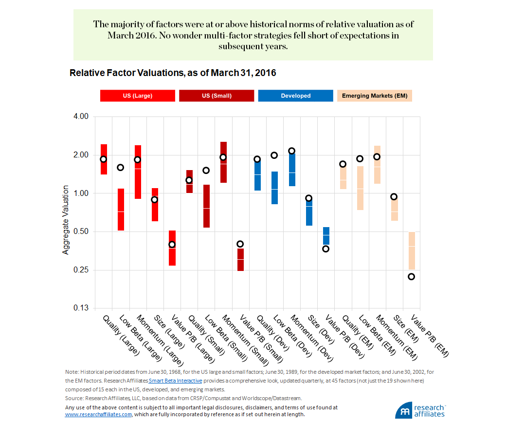
Each bar also has a white dash roughly in the middle of the bar, and a circle. These represent the prior median relative valuation for each factor, and the then-current relative valuation as of March 2016. For quality, by happenstance, the circle on the bar rests on the median line (actually slightly below it). In March 2016, high-quality US large-cap stocks were priced at an average premium of 84% relative to low-quality stocks; this was very near the long-term historical median premium of 90%.
We apply the same method to the other factors, showing that seven of nine factors in the US market were at or above historical norms of relative valuation as of March 2016. No wonder US multi-factor strategies fell far short of expectations – most failing to add any value at all – in the subsequent five years! It bears mention that the practitioner community encouraged those lofty expectations, often with the use of historical simulations, some showing that multi-factor strategies should never underperform over a three- or five-year span.
We observe a clear link between cheapness relative to history and subsequent factor performance.
”In March 2016 quality, low beta, momentum, and size were all trading at substantial premiums on a relative valuation basis across the developed markets, and value was trading at a discount in all non-US regional markets. We can think of valuations far removed from the historical median as a stretched rubber band, which history shows tend to snap back; in other words, the relative valuations tend to mean revert.
Extending the rubber band analogy, we convert each of the March 2016 relative valuation measures to a Z-score (log scale), which measures how far the rubber band was stretched away from historical norms. Fifteen5 of the 19 factors were trading rich, above historical norms. Nine6 of the 15 not only failed to match their historical success, but actually hurt investors over the subsequent six-and-a-half years. These results are before any trading costs, fees, implementation shortfall, or any other element of slippage, all of which erode returns (Arnott, 2006).
Of the four factors trading cheap in March 2016, two (US large quality and EM value) added value in the subsequent six-and-a-half years. Only one was a US strategy. The remaining seven of the nine US factors were trading rich, and five out of the seven hurt their investors. Is it any wonder that multi-factor strategies fell short of investors’ expectations?
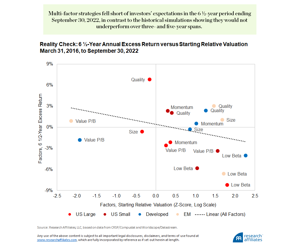
We observe a clear link between cheapness relative to history and subsequent factor performance. For any given year, the relationship is weak, but over longer spans, it is surprisingly strong. The diagonal dotted line in the preceding figure shows that each one-sigma shift away from historical norms was worth about 110 basis points a year in relative performance for the 6 1/2-year period ending September 30, 2022. While this sounds modest, it’s not: the quintile with the lowest relative valuation beat the quintile with the highest by 570 basis points per annum for 6 ½ years, a cumulative performance gap of 3700 basis points. It also bears mention that the intercept on the graph, at a Z-score of zero, is approximately 44 basis points a year. While this is far short of historical norms, it is positive! Factor investing has merit, even if the evidence of the last several years is not encouraging.
… This Is Now
Fast forward six-and-a-half years. We repeat our earlier relative-valuation comparison of March 2016, but for September 2022. We note that low beta has swung from very expensive to very cheap for US large-cap stocks, as has momentum. And over the last six-and-a-half years, quality beat performance expectations, in part because high-profitability stocks became more expensive relative to low-profitability stocks7, leaving quality as the most expensive US factor today. Value fell far short of expectations, in part because value stocks got much cheaper relative to growth stocks, leaving US large-cap value at the 15th percentile of historical relative cheapness for the value factor.

In a near-perfect mirror image of the situation in 2016-17, of the nine US factors, seven (large low beta, large momentum, large size, large value, small quality, small momentum, and small value) are now trading cheap relative to history, with six of the seven in the cheapest quintile of the historical range. Only two are trading rich relative to history and neither is in the top quintile. Of the 19 factors worldwide, 14 are trading cheap, with 11 in their historically cheapest quintile ever (US large low beta, US large momentum, US large size, US large value, US small quality, US small momentum, Developed momentum, Developed value, EM low beta, EM momentum, and EM value). Of the five factors that are trading rich relative to history, only one—quality in the developed markets—is in the top quintile of historical relative valuation; this preference for quality is likely a direct consequence of the geopolitical shocks currently threatening Europe and Japan.
Factor investing has merit, even if the evidence of the last five years is not encouraging.
”We like to buy when the market is at “peak fear.” That fear creates the very bargains we are measuring here and drives the very narratives that discourage people from buying. In short, when money was pouring into multi-factor strategies in 2016-17, it proved to be a terrible time to embrace these strategies. In 2022, after a protracted period of disappointing returns and elevated economic and capital market uncertainty, performance chasing means investors are turning away from poorly performing multi-factor strategies. Yet, as these multi-factor strategies shed assets at a prodigious pace, today most factors do not merely look cheap, they look very cheap!
Performance chasing is addictive. When we published “Horribly Wrong,” some of the trendiest smart beta factors and strategies had enjoyed soaring relative valuations, which amplified both their past returns and the consequent risk of future mean reversion toward historical norms. Not surprisingly, many of these strategies were enjoying massive inflows at the time. We suggested then that investors might see their expectations dashed in the performance of the most beloved smart beta factors, contrary to the backtests rolled out by many smart beta strategy vendors. Today, we believe the caution we urged in 2016-17 no longer applies.
Alas, we cannot see the future. But if the relationship between relative valuation and performance is as powerful over the next few years as it was since 2016-17, the 11 factors trading in the cheapest quintile of historical relative valuation should beat the five that are trading rich by perhaps 1000 basis points over the next five years—a worthy margin of victory.8 Now appears to be a particularly promising time to embrace multi-factor investing.
The Factor Investing Nadir
Value investing hit its nadir during the summer following the advent of Covid, almost exactly at the end of August 2020. No one knew how long lockdowns would last. Nor could we know how much of the economy was headed for bankruptcy (almost all of this narrative aimed directly at value stocks) or how long the wait would be for an effective vaccine. We, as well as others, observed at the time that by some measures growth had never been as frothy relative to the broad market, nor value as cheap, even at the peak of the 2000 dot-com bubble.
Using the Fama–French value factor,9 the spread between growth and value very nearly reached a tenfold relative valuation in March 2000 against a historical norm of about 4½-fold. By the end of August 2020 that spread had widened to nearly 13-fold. We noted then that this meant the value spread had set a new record, with growth 30% richer relative to value than at the peak of the dot-com bubble. Of course, it would have been easier at that time to persuade investors to sample strychnine than to rebalance into value!
At the end of August 2020, value was far from the only factor trading at extremes. Exactly how extreme is indicated by the fact that we had to expand the scale of the next exhibit fourfold (!) to encompass the extraordinary outliers. A portfolio of the 30% of stocks with the greatest momentum was trading at a relative valuation 5.7 times—an all-time high—that of a portfolio holding the 30% worst-momentum stocks. This 470% premium was eight times as large as the historical norm of 60%. Quality was in the top decile of relative valuation in all market segments but US small-cap. Low beta was in the top percentile of relative valuation in the US market. Size (small-cap versus large-cap) was trading well into its cheapest decile in the US market. Indeed, 15 of the 19 factors were in either their richest or cheapest decile in history, with 6 (US large low beta, US large momentum, US large value, Developed value, EM momentum, and EM value) in their most extreme percentile ever.

With the caveat that we are cherry picking our starting point—the most extreme market conditions in history for many factors—how have these factors performed since then? The 10 factors in their richest decile in history as of August 31, 2020, lost an average of 8% over the subsequent 25 months. The 5 factors in their cheapest decile ever earned an average of 41% in the same brief time span. The 4 midrange factors earned an average of 5% in the same time period. The very extreme relative valuations we witnessed in August 2020 led to a −73% correlation between the stretch of the valuation rubber band (its Z-score) and subsequent 25-month performance, as we can vividly see in the next graph. Yes, Virginia, there is a link between the relative cheapness of a factor and its subsequent return; that linkage becomes stronger when we find ourselves with extreme outliers. Indeed, each one-sigma change in relative valuation was worth 395 basis points per annum in the two short years since value found its all-time record lows.

A Wake-Up Call for Academia and for Practitioners
Our analysis reaffirmed the powerful link between relative-valuation multiples and the subsequent performance of almost all factor strategies we tested. This utterly unsurprising finding, while well documented in stocks and many other asset classes (in stocks, we know it as the value factor), is viewed with skepticism in the realm of factor investing, quant strategies, and so-called smart beta. How could it not be smart to use the factors and strategies with the best past performance? Isn’t that completely different from the performance-chasing that so many investors pursue?
As a result, many investors often gravely underappreciate the relevance of a very simple set of questions:
- Is a long-short factor trading unusually cheap or rich relative to history, when measured by the long portfolio’s fundamental valuation multiples relative to the short portfolio (e.g., relative price-to-earnings ratio, relative price-to-book ratio, relative dividend yield, and relative price-to-sales ratio, or a blend of the four, which we use)?
- Is a long-only strategy trading unusually cheap or rich relative to history when measured by the portfolio’s fundamental valuation multiples relative to the market?
- Is a meaningful part of a factor’s or strategy’s past return partially, even largely, attributable to the changes in these relative valuation levels, rising or falling over the chosen time span for performance measurement?
- Does our preferred strategy exhibit a link between relative valuation multiples and subsequent performance?
- Do the relative-valuation multiples for the strategy exhibit mean reversion, so that soaring relative valuations or tumbling relative valuations may presage abnormally good or bad future performance, respectively?
We should not be surprised that the relative valuation of a strategy does in fact help us more accurately forecast future performance.
When we wrote “Horribly Wrong,” we hoped that investors, strategists, consultants, academics, and asset managers—especially in the quant community—would embrace the importance of relative valuations, both for long-short factors and for long-only strategies. Even if we choose to ignore the possibility of mean reversion, where high past returns can portend poor future returns, or vice versa, we should at a minimum consider whether a strategy has worked primarily because it has seen positive “revaluation alpha” (i.e., has become more expensive). This has not happened. Indeed, backtests are perhaps more widely used in marketing than ever before.
We find it disappointing and surprising that few, if any, of the scores of journal articles published in the subsequent 6½ years, introducing and examining new factors and strategies, have meaningfully explored any of the questions we pose. Shouldn’t the role of revaluation alpha, both in evaluating past returns and in shaping expectations for future returns, be a prerequisite for publication, no less relevant than the obligatory Fama–French attribution of past returns?
Now appears to be a particularly promising time to embrace multi-factor investing.
”We have often said that the most pervasive and dangerous mistakes in investing are performance chasing and data mining. This is no less true in the quant community, where the conceit is that our models, our reliance on supposedly long-term historical data, and our objective and disciplined implementation of our strategies, will surely protect us from performance chasing. Quantitative methods do not protect us from these mistakes, if we choose our strategies and models in part based on past performance. The too-common practice of using backtests to improve our backtests is the most pernicious form of data mining.
We submit that an academic seeking tenure has no better path to that goal than to identify a new factor that has generated great past performance. But where is the incentive to willingly test if the strategy owes its past performance to upward revaluation, unless that test is required in order for the research to be published? That test could force our academic to discard months of diligent work. Why would an asset manager choose to run such a test on their best-performing backtest, unless clients and consultants demand it? That test could spoil the marketing potential for a hot new product.
Can investors embrace a strategy that has massively underperformed—as a direct consequence of an even more-massive drop in relative valuation multiples—but also has the best forward-looking return expectations after adjusting for past revaluation alphas and current relative cheapness? This question is not hypothetical: Many value strategies across the regional markets, including our own RAFI™ , RAE, and RAFI MultiFactor strategies, were in this exact situation two years ago. Beating value relentlessly was no protection against client defections when value itself was bleeding red ink.
Ultimately, we urge investors and academics to commit to a few simple, critical, and often-underappreciated practices, such as netting out the effect of changing valuations, rebalancing into disappointing factors or strategies and out of the biggest winners, and adjusting expectations to allow for the possibility of mean reversion to historical norms. These choices, which may seem simultaneously intuitive and unconventional, and at times may steer us towards uncomfortable choices, offer a surer path to investment success. These guiding principles hold true for the past, the present, and the future.
Appendix: The 2016 Controversy
Our paper was critiqued by some competitors—the best-known being Cliff Asness (2016). My initial reaction was a blend of irritation and amusement. In due course, I was grateful!10
My coauthors and I were amused that the paper stirred such controversy, given the banality of our findings. Suppose a stock’s price-to-earnings ratio doubles against flat earnings. Obviously, the stock doubles. Suppose we had written a paper suggesting that this stock’s lofty past return includes a presumably nonrecurring doubling of its price-to-earnings ratio, is therefore a poor predictor of its future returns, and that any mean reversion in valuation multiples could turn high past returns into poor future returns. Suppose we had asked the question, “should we be excited by the 100% gain or uneasy that valuations have doubled relative to the underlying fundamentals?” Suppose we showed that relative valuations in stocks exhibit long-horizon mean reversion and that recent momentum offers only a short-term tailwind. The reaction would have been correctly dismissive: “Everyone knows that!” By making identically the same observations about investment strategies and factors, we apparently kicked a hornet’s nest.
Consider a strategy that soared over a 10-year period from a valuation multiple that matched the market multiple to a 100% premium. All else equal, that shift in multiple would produce 7% annual outperformance.11 Suppose the strategy beat the market by 5% a year during that decade. Investors would likely applaud its brilliance, and countless billions in investor capital would likely flow into the strategy. But, if that 5% outperformance was more than entirely explained by its 7% upward revaluation, then perhaps there’s no structural alpha at all. If a strategy becomes massively more expensive, this upward revaluation is, at best, a source of past return that we cannot rely on in the future. Worse, given any mean reversion in valuation multiple of the strategy, the wonderful past returns for the strategy may have set the stage for dreadful future returns.12 This is not a hypothetical scenario. It is exactly what happened in the 6½ years since we published “Horribly Wrong”; and, it is exactly what happened in the two years since the value factor nadir of August 2020.
History has shown that our core observations remain as true today as in 2016–17. Critics have become more subdued, although our current revisiting of the “Horribly Wrong” paper may change that. In any event, controversy is our friend. It helps us better understand how the world works. Investing is nothing if not a continuous life-long education for those who are receptive to new ideas and to learning.
Please read our disclosures concurrent with this publication: https://www.researchaffiliates.com/legal/disclosures#investment-adviser-disclosure-and-disclaimers.

Endnotes
1. At year-end 2016, our forecasts for the low beta factor across all regions ranged from −1.5% to −2.5%. In the subsequent five years, the factor indeed suffered losses ranging from 1.8% (developed market) to 4.9% (US market). Back then, we also counseled caution in the size and illiquidity factors in US and developed stocks; the returns for these two factors also fell by −2.5% or more a year five years hence.
2. In our 2016 “Horribly Wrong” article, we called revaluation alpha “situational alpha.” After a client suggested “revaluation alpha” as being a far-more intuitive name, we have used it ever since. The residual, after revaluation alpha, is a blend of structural alpha and noise. The latter is typically dominant.
3. The definitions and calculations of each factor are available in Methodologies Used in the Interactive Smart Beta Tool, available on Research Affiliates Smart Beta Interactive.
4. The careful reader may notice that the start date of the analysis in this paper (June 30, 1968) differs from the start date listed in the original “Horribly Wrong” paper (January 1, 1967). A variety of reasons contributed to this inception date shift, including but not limited to, data quality improvements, rebalancing shifts, and competitor-portfolio consistency considerations.
5. The 15 factors trading rich were US large low beta, US large momentum, US large value, US small quality, US small low beta, US small momentum, US small value, Developed quality, Developed low beta, Developed momentum, Developed size, EM quality, EM low beta, EM momentum, and EM size. We analyze here 19 factors rather than 20 (i.e., five strategies in four regional markets) because there is no size factor for US small; this factor measures small versus large.
6. The nine factors that negatively impacted investor performance over the six-and-a-half-year period from March 2016 to September 2022 were US large low beta, US large momentum, US large size, US large value, US small low beta, US small value, Developed low beta, Developed size, and EM low beta.
7. Quality moved from a relative valuation of 1.84 in March of 2016 – meaning high-profitability stocks traded at an 84% premium relative to low quality stocks – to a relative valuation of 2.16. Ignoring the role played by changing composition of the high and low quality portfolios, this 17% rise in relative valuation would suggest a revaluation alpha of 2.7% per year, contributed just under half of the 6.8% positive performance of the quality factor during the 6½ years.
8. The eleven factors that are trading in their cheapest quintile are an average of about 1.31 sigma cheap. Those that are trading rich are an average of about 0.43 sigma rich. Given that the annual subsequent performance seems to be 1.1% per one-sigma difference in the starting relative valuation, this 1.74 sigma difference should point to 957 basis points of relative performance (1.1% x 1.74 sigma x five years), albeit with considerable uncertainty. For example, the far stronger linkage between starting z-score and alpha since August of 2020 suggest that this may be a substantial underestimate.
9. The Fama–French value factor selects the 30% of US large-cap stocks with the highest book-to-price ratio and the 30% of US small-cap stocks with the highest book-to-price ratio then puts half into each of these capitalization-weighted lists to create a value portfolio. The growth portfolio consists of the 30% of the US large-cap market with the lowest book-to-price ratio, cap-weighted within that list and equally weighted with the 30% of the US small-cap market with the lowest book-to-price ratio.
10. We are grateful that a respected thought leader chose to provide a detailed review of one of our papers. Many observations were highly valuable in improving our understanding of the nature of revaluation alpha and identifying better ways to turn the findings into incremental performance.
11. Of course, all else is not equal. We need to be particularly careful with high-turnover factors and strategies, such as momentum or low beta, for which the portfolio may trade from low-valuation to high-valuation stocks without earning revaluation alpha.
12. This is not, and never was, the same as advocating aggressive factor timing or highly concentrated bets in individual factors.
References
Arnott, Robert. 2006. “Implementation Shortfall.” Financial Analysts Journal, vol. 62, no. 3 (May/June): 6–8.
Arnott, Rob, Noah Beck, and Vitali Kalesnik. 2017. “Forecasting Factor and Smart Beta Returns (Hint: History Is Worse than Useless).” Research Affiliates Publications (February).
Arnott, Rob, Noah Beck, Vitali Kalesnik, and John West. 2016. “How Can ‘Smart Beta’ Go Horribly Wrong?” Research Affiliates Publications (February).
Asness, Clifford S. 2016. “The Siren Song of Factor Timing aka ‘Smart Beta Timing’ aka ‘Style Timing.’” Journal of Portfolio Management Special QES, Invited Editorial Comment, vol. 42, no. 5:1–6.
