
Alternative risk premia strategies can play an important role in an investor’s portfolio, providing an additional source of diversification when traditional headline asset classes go through tumultuous periods (e.g., 2022).
Investors should be wary of hidden exposures to headline asset class risk factors lurking under the surface and not be misled by the low correlations measured over the long term.
A risk-neutral portfolio construction approach can significantly reduce the unintended bets taken by a dollar-neutral approach and maximize the diversification benefits of alternative risk premia strategies.
Introduction
The 2022 broad market downturn across major asset classes came as a nasty surprise to investors. Historically, such an event is very rare, and no one was expecting to see almost all asset classes down for the year. Yet, even though it might seem as if diversification was of no help in 2022, the story changes if we look beyond the major headline asset classes.
For the year, alternative risk premia strategies actually posted modest gains on average. In that respect, the 2022 experience provides a good reminder that investors should consider diversifying their portfolio of headline asset classes through alternative risk premia strategies that harvest returns orthogonal to those of traditional asset classes. At least that’s how the investment landscape looks on the surface, but that appearance is deceiving.
Create your free account or log in to keep reading.
Register or Log in
Below the surface, hidden risks lurk unseen and ready to emerge. In fact, investors would do well to learn a lesson from the classic science fiction novel Dune (and its recent movie adaptations). On the desert planet of the title, nomadic inhabitants known as Fremen must live with the constant threat of being devoured by giant predatory sandworms (called Shai-Hulud) that tunnel through the dunes. The worms are attracted by the sound of rhythmic movements. The Fremen have survived by developing two strategies. The first is a shuffling, dance-like sand-walk that disguises their movements. (In our nonfictional world, surfers have developed an analogous wading technique called the stingray shuffle.) The second strategy is learning how to read the subtle wormsigns on the sand that provide advance warning of an approaching Shai-Hulud.
Like the desert-dwelling Fremen, investors who want to reap the gains of alternative risk premia strategies would do well to learn how to adapt to unseen risks—hidden exposures to headline asset class risk factors. As our analysis shows, practical techniques of portfolio construction can mitigate such risks. We must learn to shuffle through shifting sands and read the wormsigns.
Like the desert-dwelling Fremen [from Dune], investors who want to reap the gains of alternative risk premia strategies would do well to learn how to adapt to unseen risks.
”Revisiting the Role of Alternatives
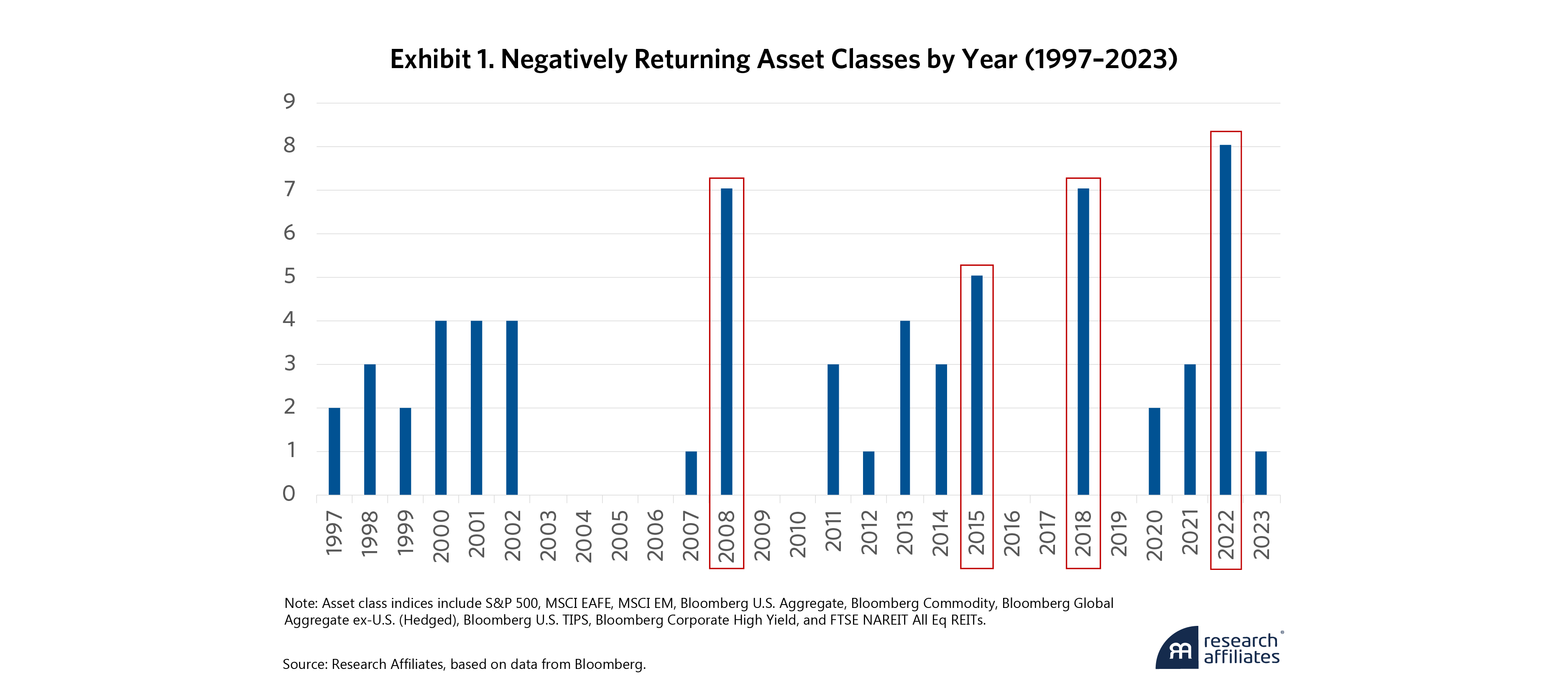
As noted, 2022 was a particularly painful year. Among headline asset classes, only commodities were up for the year, reflecting high inflation. Furthermore, as of the end of June 2024, certain asset classes, such as bonds, have yet to dig out of the 2022 drawdown (indeed, Bloomberg U.S. Aggregate Bond Index is still in a drawdown of approximately 9% since the beginning of 2022). In Exhibit 1, if we look at the calendar returns of nine indices that represent a broad range of headline asset classes, it is unusual to see a calendar year where more than half (five) of the indices post negative returns. In fact, it has occurred only four times in the period from 1997 to 2023.
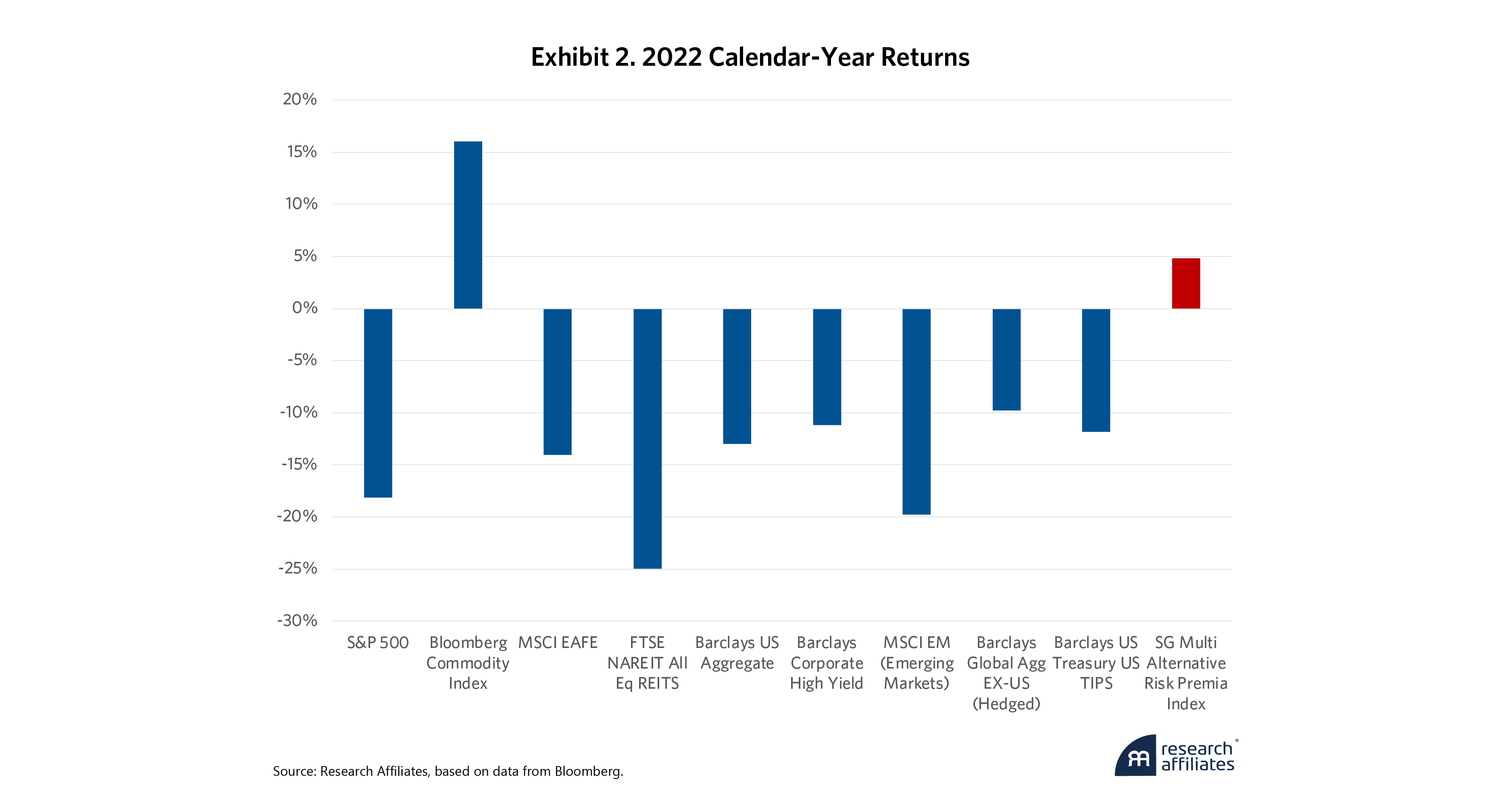
Given this context, the gains of alternative risk premia strategies provide a stark contrast. For example, the SG Multi Alternative Risk Premia Index, an index composed of alternative risk premia funds, produced a gain of approximately 5%, as displayed in Exhibit 2.
Having written about the role of alternative risk premia strategies as part of an investor’s broader portfolio (Ko, Kunz, and Shepherd 2018), we believe the recent experience of the 2022 downturn provides an instructive opportunity to revisit this topic. The key takeaway is that incorporating a meaningful allocation to alternative risk premia strategies can improve an investor’s future investment outcome by increasing the likelihood of clearing return hurdles while helping to reduce portfolio volatility and other higher-order risks (e.g., skew).
However, given the various components and potential complexities of alternative risk premia strategies, we must also acknowledge that these strategies may pose risks of their own. Like the nomads of Dune, we must shuffle our feet through the sand to avoid the hidden risks that may be hiding under the surface of these strategies. It is important to lay out a robust framework for building an alternative risk premia strategy, starting from the universe, signal, and portfolio construction. The investment industry and academia have concentrated much attention on identifying new risk premia signals (factors), but this article focuses on an area often taken for granted: portfolio construction. For more on factor “zoo” literature, see Hsu and Kalesnik 2014 as well as Feng, Giglio, and Xiu 2020.
Constructing Risk Premia Portfolios
Across finance literature, portfolio construction of cross-sectional long-short risk premia portfolios generally follows a similar framework as summarized here:
- Measure the risk premia signal of each asset within a defined universe.
- Sort and rank the assets by value of the signal.
- Assign top (bottom) x% of the assets to long (short) leg.
- Within a long or short leg, assets can be weighted in various ways (e.g., equal weighted, rank weighted, etc.).
- Long and short legs are sized equally so that all weights sum to zero (dollar-neutral). For example, long (short) assets sum to 100% (-100%).
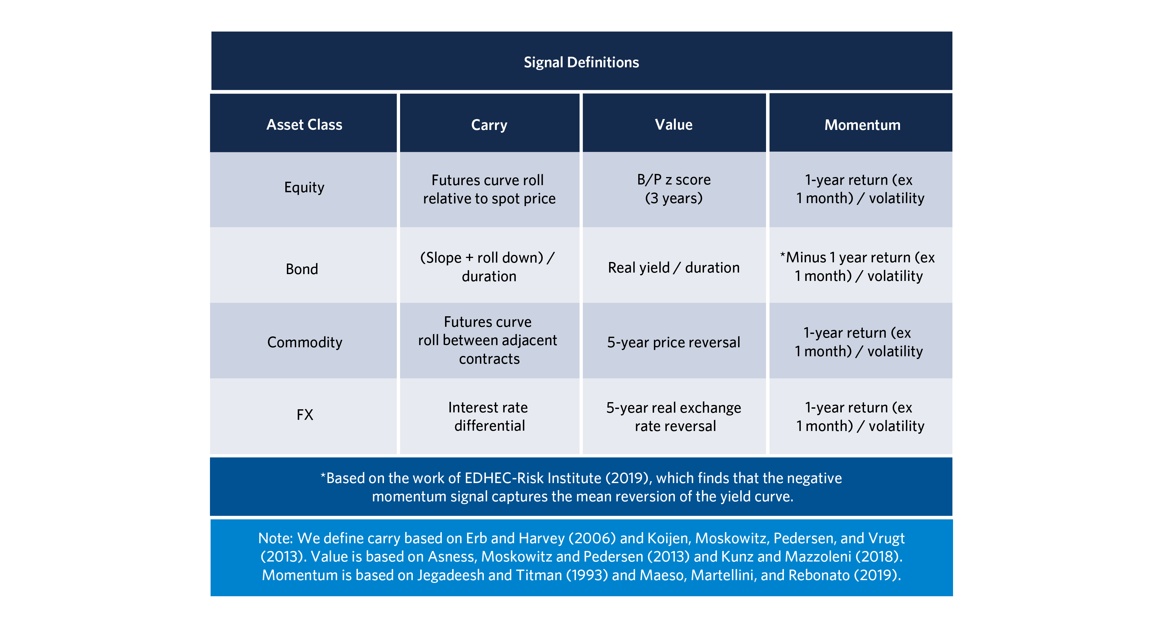
For the purposes of this article, because the focus is not on identifying the best signal or assets, we use a set of well-cited risk premia signals (carry, value, and momentum) across familiar asset classes (equities, bonds, commodities, and FX), building on Brightman and Shepherd (2016). Assets include 15 equity index futures, 17 government bond futures with maturities ranging from 2 years to 10 years, 27 commodity futures, and 15 FX forwards denominated against the U.S. dollar across both developed and emerging markets. To avoid data-mining concerns, we have chosen signals based on definitions that are relatively simple and have been found to be robust.
The simulation spans December 1999 through March 2024, and we construct 12 individual risk premia strategies and also create aggregate strategies, both within and across asset classes. All portfolios are rebalanced at month-end. When forming the portfolios, we use tertile sorts (i.e., top and bottom 33.3%) and equal-weight the assets within the long or short leg of the portfolio. Finally, simply for comparability, we scale the portfolios ex post to have full-sample volatility of 10%. When building blended asset class strategies (e.g., blend of equity carry, equity value, and equity momentum) and the aggregate strategy (i.e., blend of equity blend, bond blend, commodity blend, and FX blend), we equal-weight the underlying strategies. Given that we first scale each strategy to 10% volatility, this approach can then be interpreted as a form of equal-volatility weighting of the strategies (of course, we would not know this volatility during trading: this simple approximation is made only for the purposes of this article).
Dollar-Neutral: What Can Go Wrong?
Portfolios that seek to harvest risk premia often reflect what is referred to as dollar-neutral portfolio construction. This approach, which takes an equal-sized position in both the long and short legs of the portfolio, was likely inspired by the long history of finance literature that utilizes “self-financing” (e.g., sell $1 of asset A to buy $1 of asset B) factor or arbitrage portfolios. Given the simplicity and economic interpretation, it is easy to see why this approach has been widely utilized by both academics and practitioners. In addition, the simplicity also improves the reproducibility of results and is likely a significant reason why so many studies in finance literature build on one another.
While simple in its implementation, dollar-neutral construction can often lead to portfolios that take on unintended (and often undesired) bets. This effect is especially likely when the underlying assets used to form the portfolio exhibit a wide range of risk characteristics. For example, consider a formation period for a commodity long-short portfolio in which the assets in the long (short) leg happen to exhibit high (low) beta to the Bloomberg Commodity Index. By construction, the portfolio would reflect a net-long directional bias to the index. Would this bias be desirable? We think not, especially because a directional commodities view can easily be achieved by overweighting the asset class through the asset allocation process. The same holds for the opposite case, a net-short view.
While simple in its implementation, dollar-neutral construction can often lead to portfolios that take on unintended (and often undesired) bets.
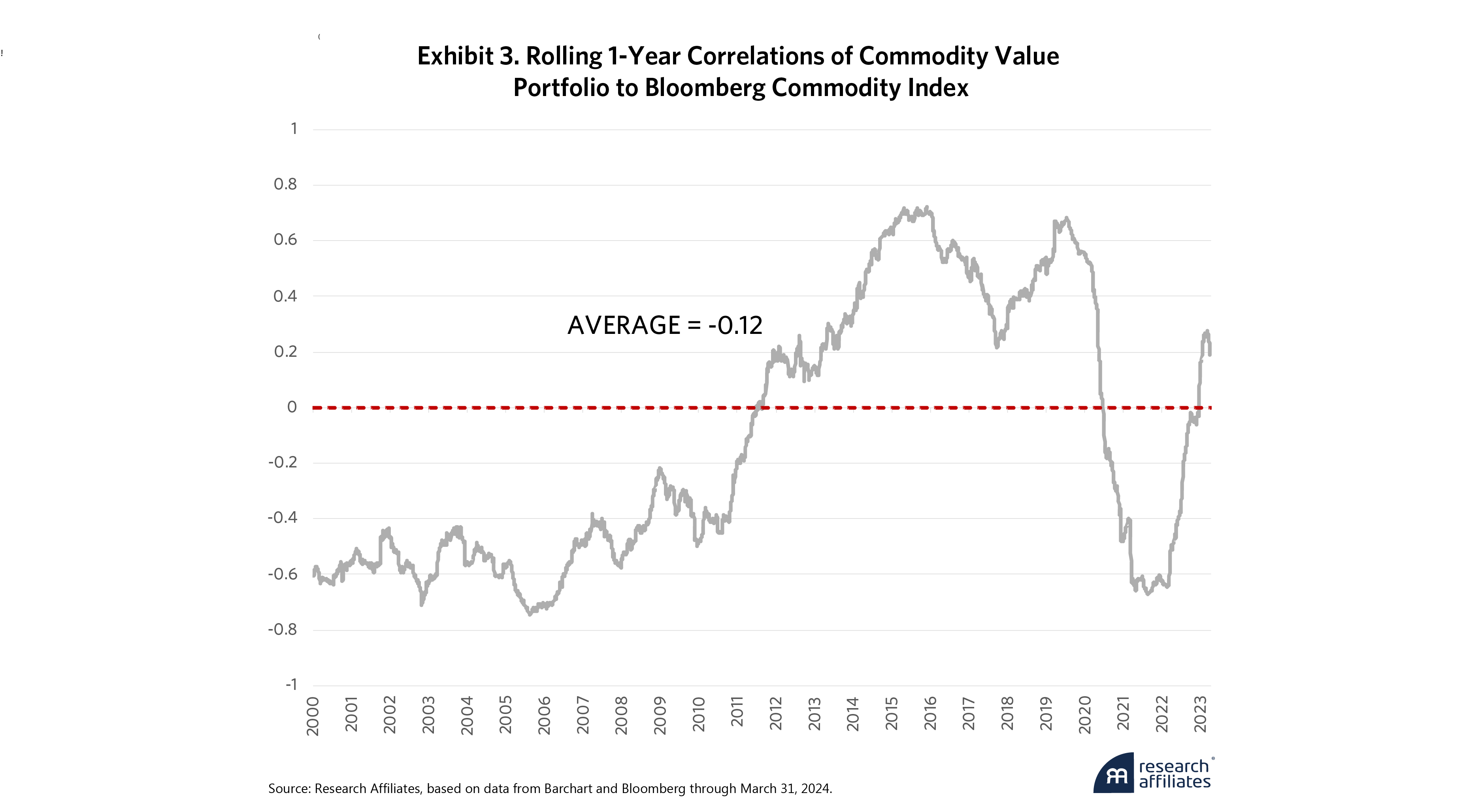
”For example, in Exhibit 3 when we measure the rolling 1-year correlations of the commodity value portfolio, we observe that it can at times be highly (both positively and negatively) correlated to the headline commodity index (see Appendix B for an explanation of how we estimate ex-post rolling correlations). As a result, the portfolio’s full-sample average correlation of -0.12 can be misleading in the sense that what the investor would experience over the simulation period likely would not reflect this single value. In fact, for extended periods, the investor might wonder, “Why is this supposedly orthogonal strategy moving in the same (or opposite) direction of the commodities market?”
The Risk-Neutral Shuffle
Many researchers have written about unintended bets that can inadvertently be expressed by a portfolio and about ways to avoid such bets, exemplified by the works of Aghassi, Asness, Kurbanov, and Nielsen (2011). As shown above, simply looking at long-term averages can give a false sense of security by hiding the high-correlation periods that emerge from time to time. In the context of alternative risk premia strategies, which bets or risks should be avoided? Regional bets? Other factor bets?
There are many ways to go about dealing with this problem, but in this article, we focus on neutralizing the underlying market risk of the asset class. In this respect, reiterating the goal of alternative risk premia strategies and their roles as part of a broader portfolio helps provide strong motivation to build risk-neutral portfolios that have hedged the directional exposures to headline markets that can be easily obtained cheaply.
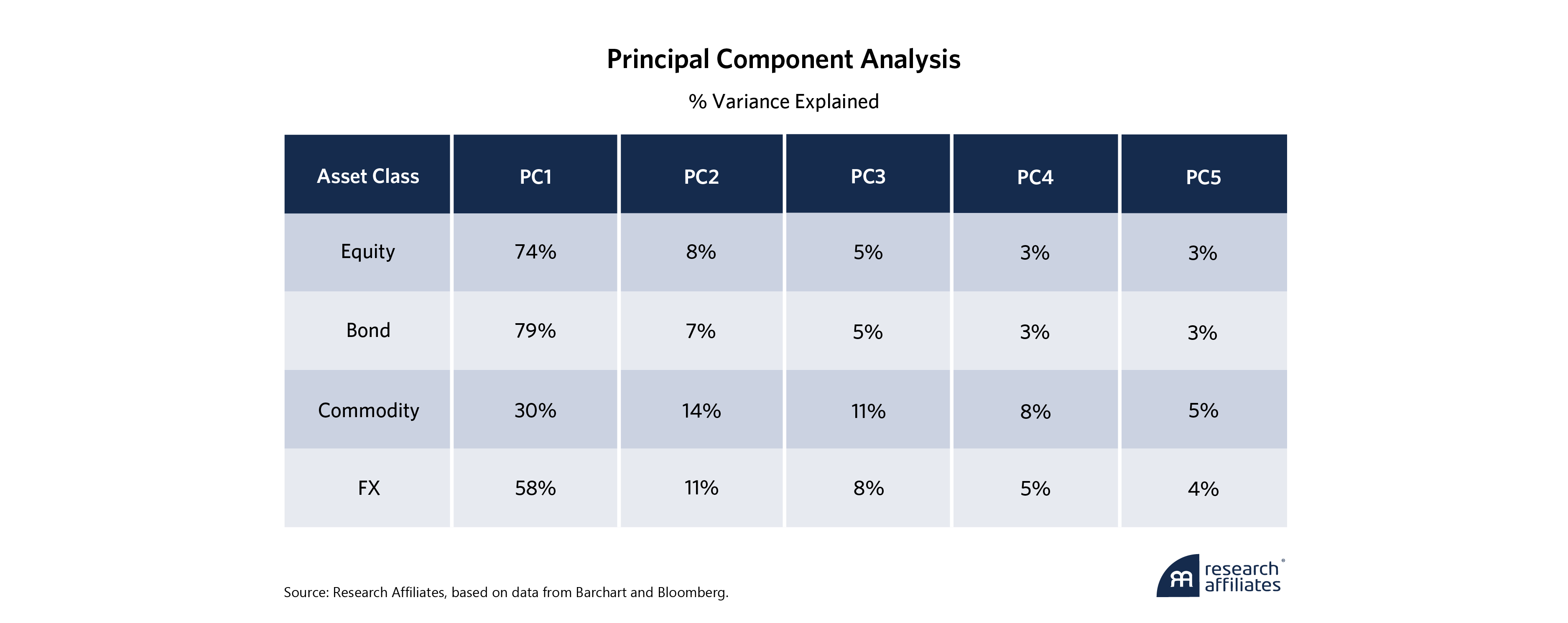
How do we know what is the underlying market risk for each asset class? To provide an answer, we use economic rationale as a foundation supported by statistical analysis. In Exhibit 4, for each of the four asset classes that represent the universe of assets, we select the headline indices as the primary risk factors. This approach has two advantages: (1) simplicity and (2) representativeness for most investors’ portfolios. Principal component analysis (PCA) shows that these indices are highly correlated with the first principal components of each asset class, suggesting that our choices are robust. For more details on PCA, see Appendix A.
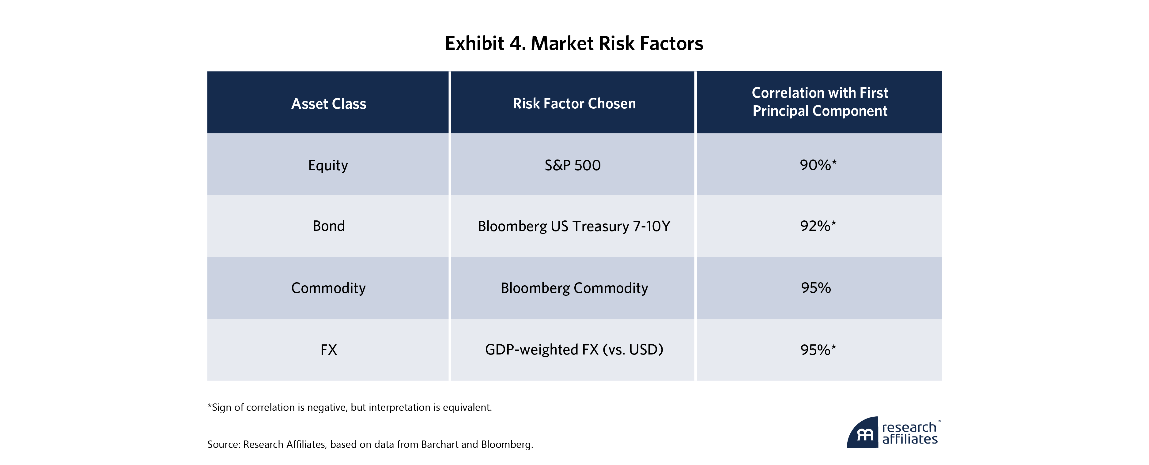
The S&P 500 represents the U.S. equity market and the intuition that it drives the global equity market. The Bloomberg U.S. Treasury 7-10 Year Index represents the underlying interest rate risk of bonds, and the Bloomberg Commodity Index represents the inflation-rate risk present in commodities, a real asset. Finally, the Purchasing Power Parity (PPP) GDP-weighted FX factor represents the global risk of the U.S. dollar.
For this article, we use a relatively simple approach for constructing risk-neutral portfolios. The first three steps are the same as the framework described above for constructing dollar-neutral portfolios, but the fourth step is replaced with the following process:
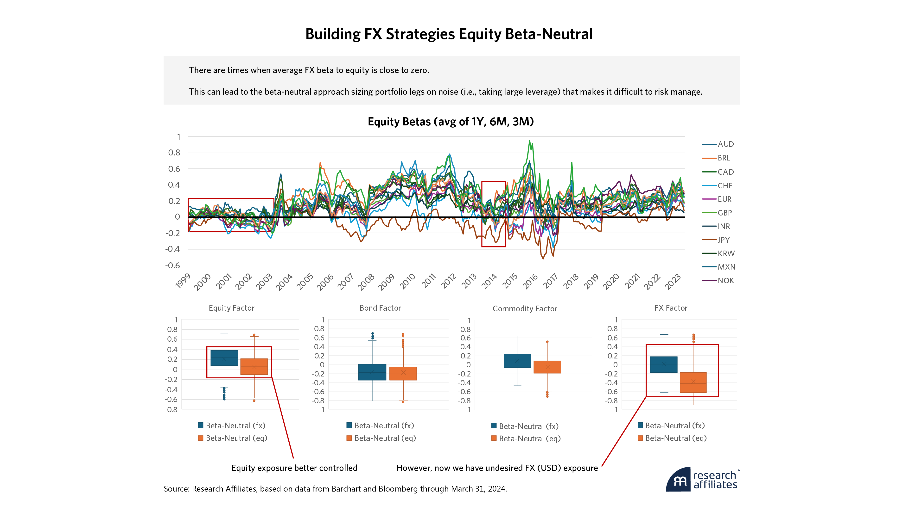
- Measure the beta of each asset to the risk factor. See Appendix B for a detailed description of beta measurement. We measure betas using trailing 3-month, 6-month, and 1-year daily data and also average these betas, which we will primarily use in the rest of the article.
- Size the long and short legs so that its weighted beta = 1.
Note that the resulting portfolio is ex ante beta neutral at rebalances by construction but may exhibit some levels of correlations to the risk factors ex post as a result of measurement noise or even as an effect of the dynamic risk characteristics of the assets themselves. For bonds, an alternative and possibly more interpretable implementation would be to construct duration-neutral portfolios. We find that both approaches give similar results; sizing the long and short legs to be beta of 1 to the Bloomberg U.S. Treasury 7-10 Year Index can be thought of as sizing the long and short legs to be duration of approximately 7 (average duration of the index).
Learn to Read the Shifting Sands
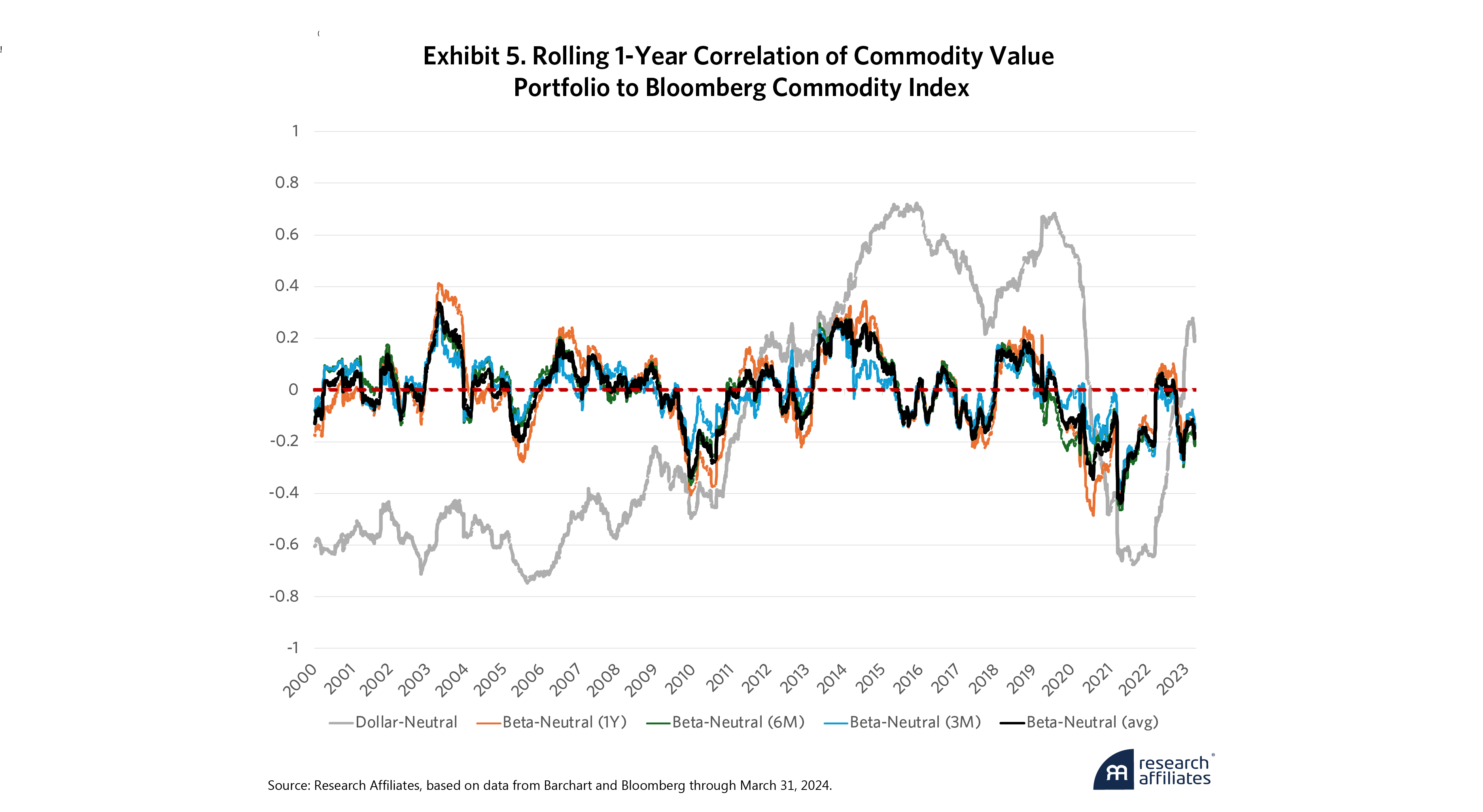
Now that we have learned the sand-walk of the Fremen, we can read the wormsigns of risks ready to emerge from beneath the surface. Again, as an example, in Exhibit 5, we repeat the same exercise of calculating the 1-year rolling correlation of the commodity value portfolio but this time include the beta-neutral versions as well. As the chart shows, the beta-neutral portfolios tend to have correlations that are centered around zero for the simulation period. In addition, the volatility of the correlations themselves also appears much lower compared with that of the dollar-neutral portfolio.
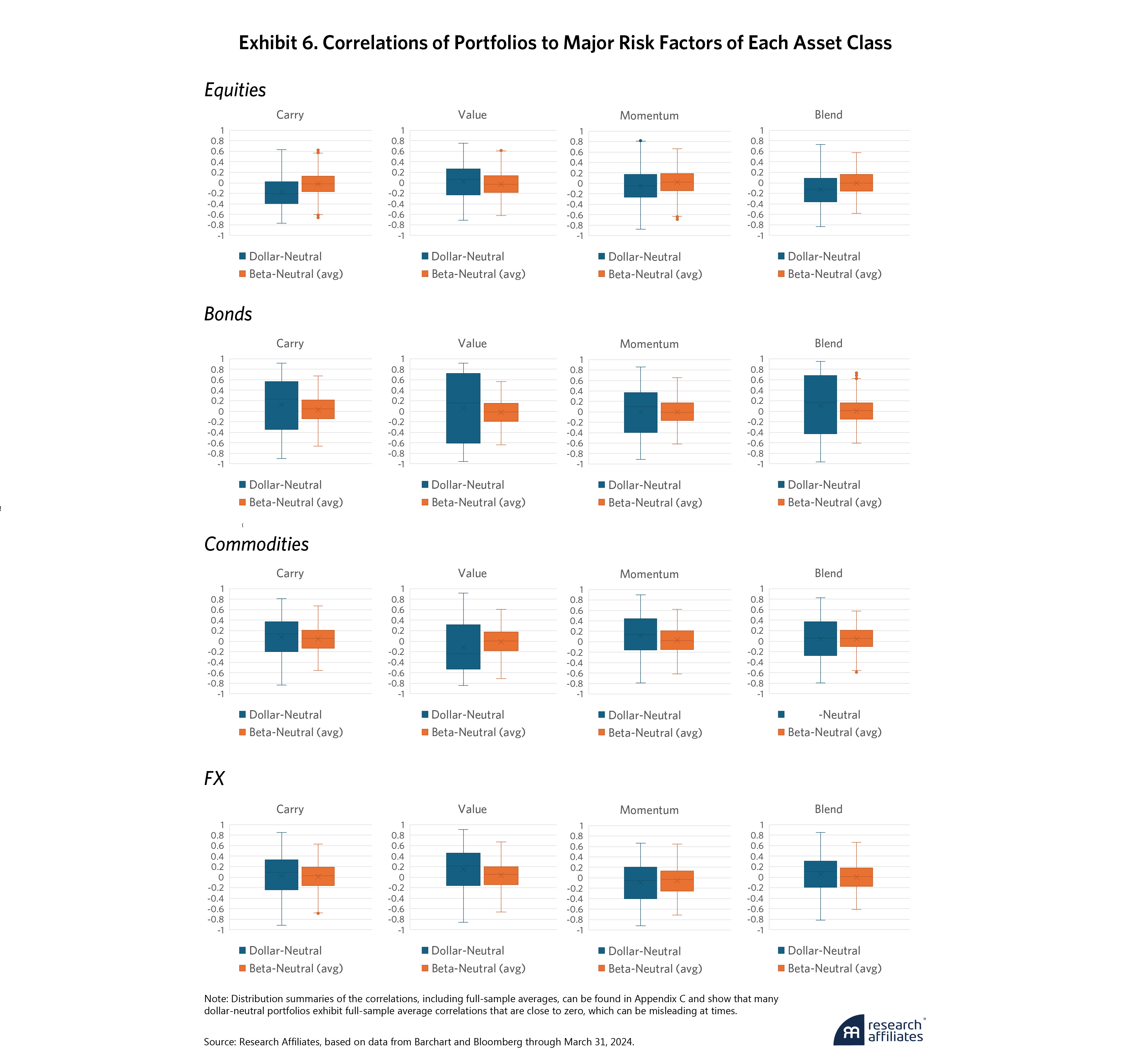
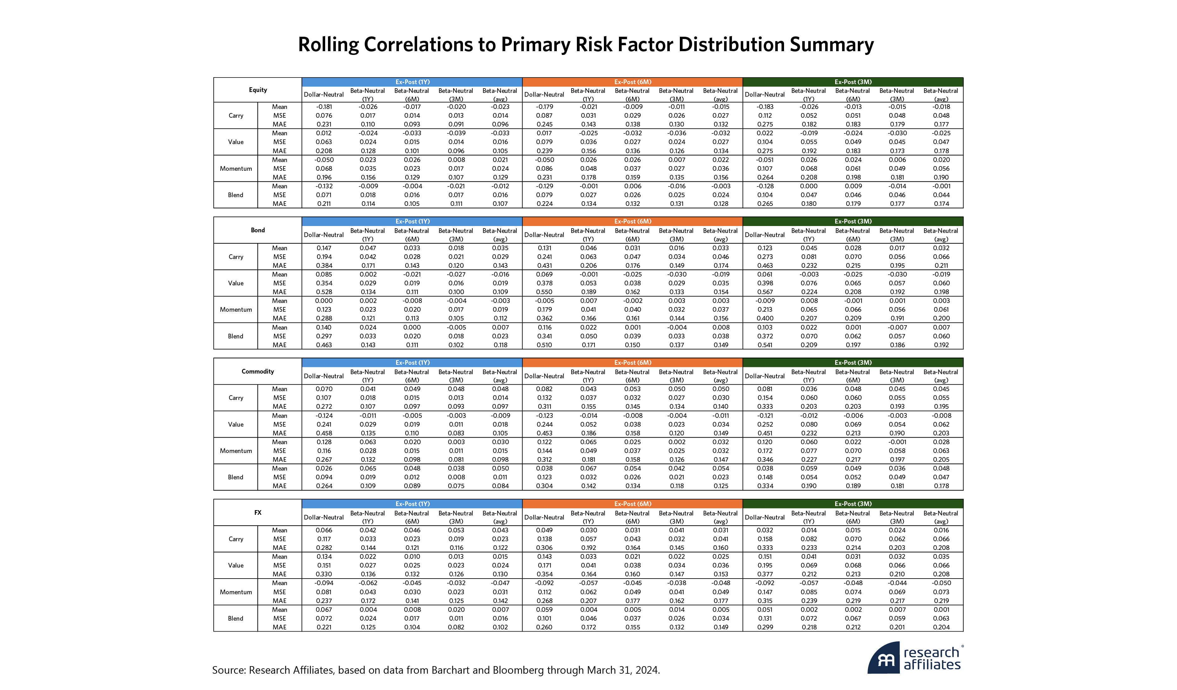
Boxplots of the rolling correlations in Exhibit 6 provide an even clearer view of the distribution differences between dollar-neutral and risk-neutral approaches. The boxplots display only the rolling 3-month correlations and only the beta-neutral portfolio that uses the average betas. Full distribution summaries can be found in Appendix C. Correlation distributions of the beta-neutral portfolios exhibit smaller ranges and outliers while being centered closer to zero on average.
Interestingly, strategies constructed on equity index futures exhibit relatively smaller differences (still meaningfully reduced) between the dollar-neutral and risk-neutral approaches. In fact, when we look at the gross leverage of the equity blend strategies, the dollar-neutral and risk-neutral portfolios have similar full-sample averages of 277% and 260%, respectively (as opposed to bond blends, which have diverging full-sample averages of 665% and 965%, respectively). This effect likely reflects the universe of equity index futures because there is not a lot of dispersion of risk among developed equity indices. Once again, the benefits of the risk-neutral approach are most evident when the assets exhibit a large range of risk characteristics.
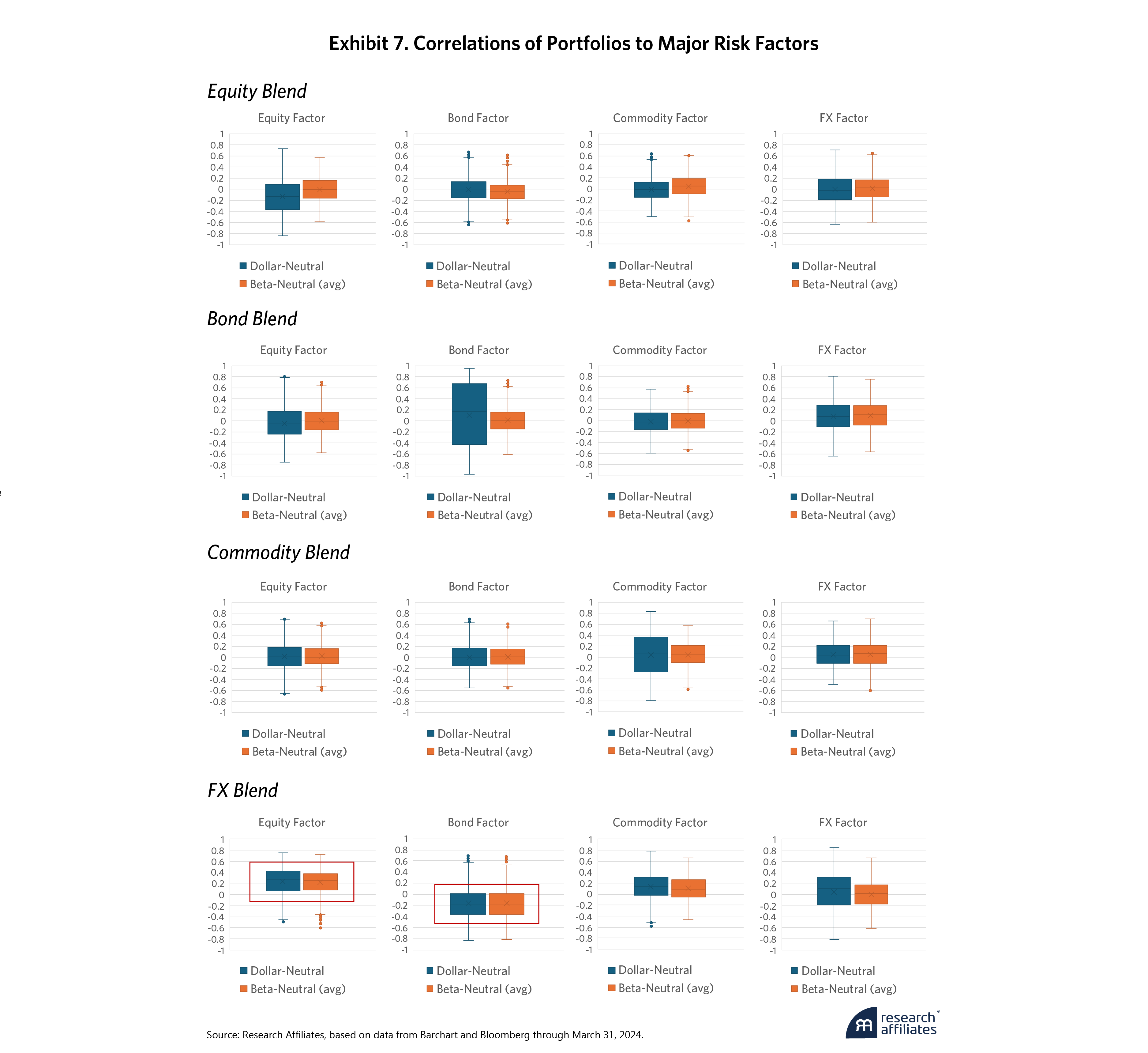
Could there be any side effects from going risk neutral? Specifically, could we be unintentionally adding exposures (yet again) to different risks by hedging one specific risk? In Exhibit 7, we look closely at each of the asset class blend portfolios by measuring the correlations not only to the chosen primary risk factors of the asset class but to all four. The boxplots of the correlations show that for most of the blended strategies, no excessive bias or volatility is observed in correlations to the non-primary risk factors specific to the asset class. For the FX blend, however, something more interesting appears: the correlations to equity and bond risk factors exhibit nonzero averages. Given that the dollar-neutral portfolio also exhibits this behavior, the appearance of these non-zero averages is likely not a side effect of the risk-neutral approach. Instead, it is likely due to the nature of the assets in the FX universe. While the GDP-weighted FX risk factor is highly correlated to (and is a good proxy for) the first principal component of FX assets, it represents only 58% of the variances of the assets. In fact, the second principal component’s correlations to the equity and bond first principal components are nontrivial at 48% and 44%, respectively. Constructing an FX alternative risk premia strategy that also hedges these other risk factors likely would require a more sophisticated portfolio construction methodology that is beyond the scope of this article, but we will touch on this point later. In Appendix D, we show that if we risk-neutralize the equity risk factor instead for all FX strategies, we can manage the equity risk better, but doing so significantly degrades our ability to manage the FX risk factor, making it an undesirable approach.
Finally, we examine the simulation performances (see Exhibit 8), a subject typically of high interest to investors but of less significance for this article. Ex ante, it is unclear what effects hedging the risk factors would have on the strategies. Compared with a dollar-neutral approach, could it improve risk-adjusted returns by better isolating the relative attractiveness of assets? Or would it instead degrade returns by eliminating the market-timing component embedded in the strategy? Even in the latter case, we believe the better approach is to construct a strategy that reflects the cross-sectional bets rather than to rely on unintentional market bets, even if it provides alpha. If there are truly any market-timing capabilities within the risk premia strategy, we believe that a better approach in a portfolio context would be to isolate that portfolio view and allocate an appropriate amount of capital or risk to it.
Several observations can be drawn from the simulation results of the various alternative risk premia strategies built using the dollar-neutral and beta-neutral approaches. First, the two approaches are highly correlated, with correlations exceeding 80% for most of the strategies (note that bond strategies have lower correlations between the two approaches, a pattern that likely reflects the wide range of risks represented in the universe, i.e., short versus long duration). This finding indicates that both approaches broadly capture similar trades and, correspondingly, portfolio returns.
Second, results for the individual strategies show a mixture of improvements (e.g., bond value) and degradations (e.g., bond carry) of risk-adjusted returns between the two approaches, reflecting the ex ante uncertainty discussed above. Interestingly, the magnitude of the degradations tends to be smaller than the improvements, leading to overall improvements for all blended strategies, but more on that later. Third, outside of equities, most risk characteristics (e.g., skew, drawdown) of the strategies are improved. Again, this result for equities is likely due to the underlying assets displaying very similar risk profiles, limiting any improvements in that regard.
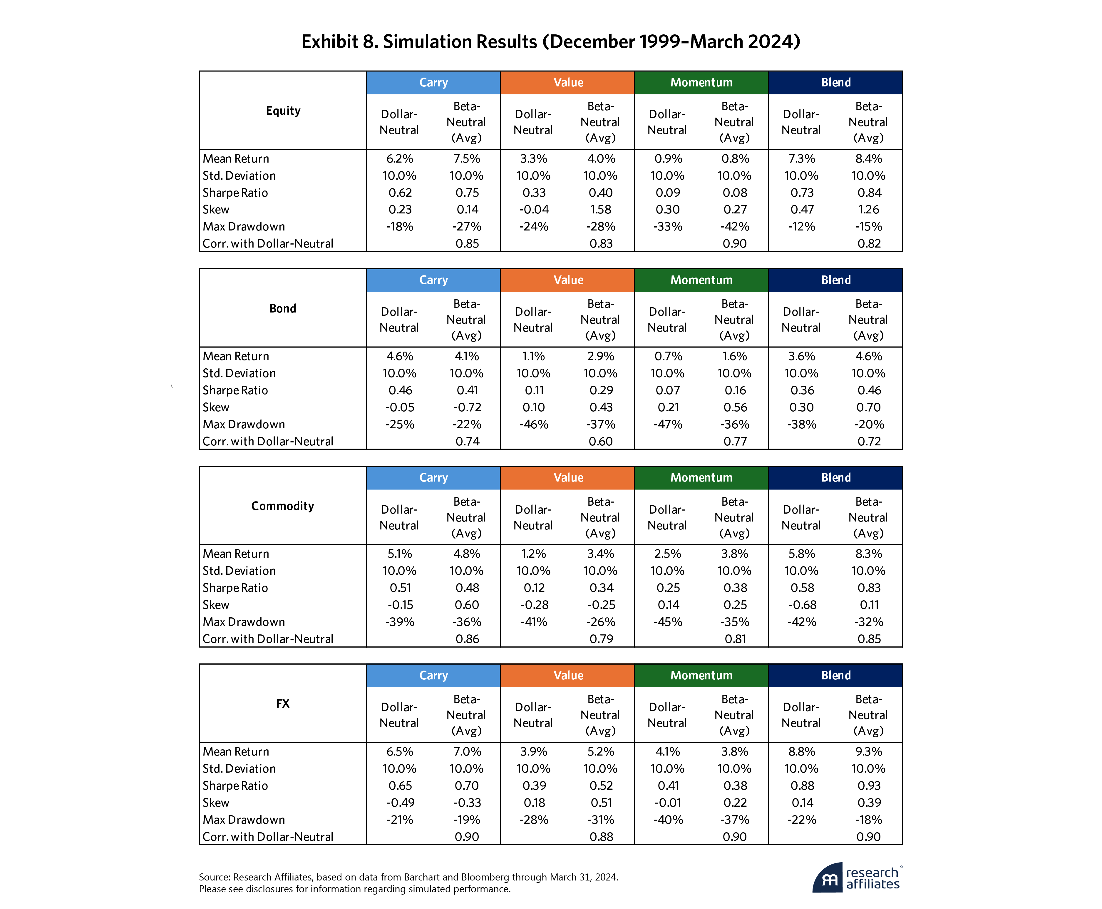
The magnitude of the performance improvements tends to be larger and more frequent than the degradations, which leads to an important question: What could be driving this tendency? The time-varying risk exposures embedded in the dollar-neutral portfolios can indeed be detractive. For example, consider both the commodity value and FX value strategies, which exhibit full-period-average risk-factor correlations close to zero at -0.1 and 0.1, respectively. The time-varying market bets of these portfolios can be isolated by measuring the residual betas at each rebalance and forming beta-timing portfolios. We find that the average returns of these portfolios are negative, with those derived from commodity value and FX value losing approximately 50 basis points (bps) and 20 bps per year, respectively. Thus, removing these market bets is likely a large contributor to why we see larger performance benefits rather than detriments from the risk-neutral strategies.
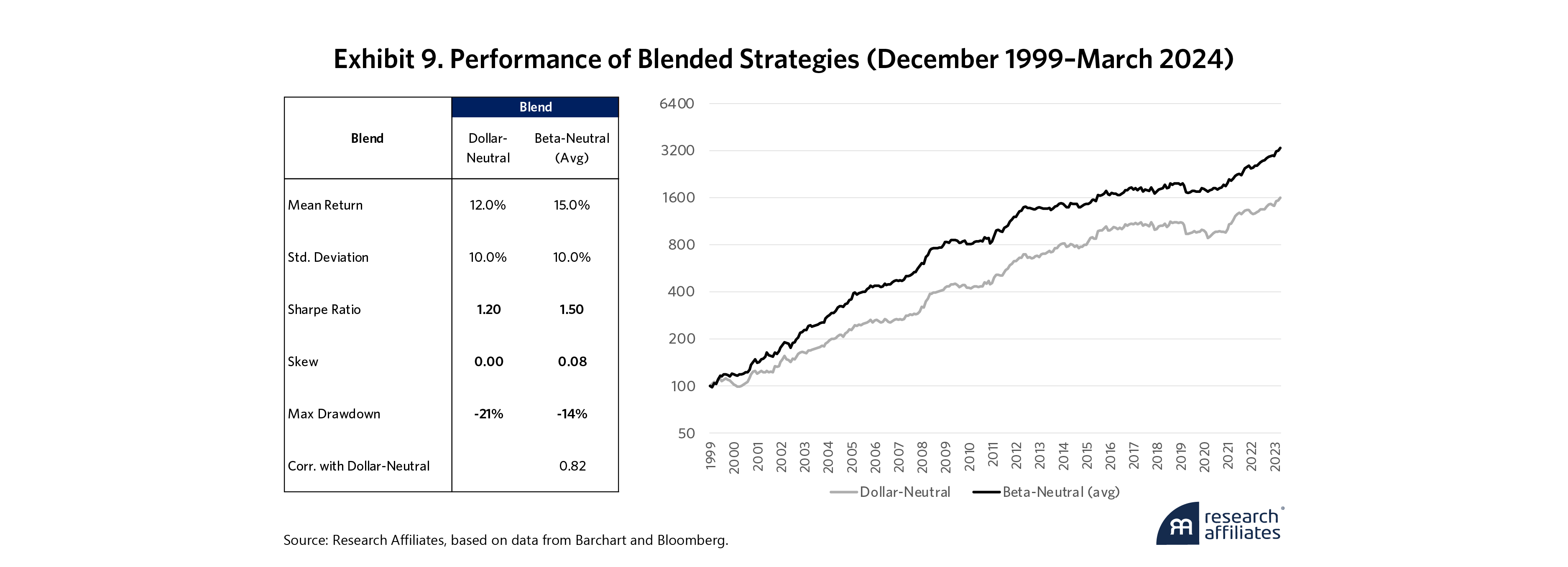
Finally, putting all the strategies together in Exhibit 9 shows a significant improvement (+0.3 Sharpe ratio) in the risk-adjusted returns and risk profile of the overall strategy. Again, these performance improvements were not the focus or the intent of the risk-neutral approach, but it is a nice benefit in addition to gaining the ability to be more intentional about the risk-factor exposures.
Conclusion
Of course, our analysis does not mean that no manager is neutralizing market risks and that we have somehow stumbled upon a novel method for risk premia portfolio construction. For many investors, especially asset managers who run alternative risk premia strategies, the points and results we share in this article may be obvious. In fact, the equity market-neutral fund industry has a long history spanning decades, and we are confident that most shops would have this dynamic figured out (it would be an issue if a market-neutral fund didn’t). Instead, this article can serve as a gentle reminder that when alternative risk premia strategies that span various asset classes are implemented, investors should consider the risk factors that such a strategy could inadvertently introduce to their portfolios and should construct portfolios with these risks in mind.
[W]hen alternative risk premia strategies that span various asset classes are implemented, investors should consider the risk factors that such a strategy could inadvertently introduce to their portfolios and should construct portfolios with these risks in mind.
”As we mentioned, the risk-neutral methodology laid out in this article is a relatively simple one. There are many extensions of the methodology that could improve managing these risk factors:
- Managing multiple risk factors: FX-based risk premia portfolios are good examples of strategies that could further benefit from managing non-primary risk factors (e.g., equity risk factor).
- Timely management of portfolio risks (e.g., betas): our method in this article is rebalanced monthly, but one could manage the risks daily and step in when either ex ante or ex post portfolio risk measures breach a threshold.
- Improving the estimation of beta or factor exposures of assets, with the caveat that one should be careful about adding too much complexity to the process.
- Alternate portfolio construction techniques and configurations: examples include optimization and sizing individual positions instead of the aggregate long or short leg, etc.
We hope to touch on these topics in future articles, but in the meanwhile, learn to shuffle through the unintended risks and—just maybe—learn to tame Shai-Hulud.
Please read our disclosures concurrent with this publication: https://www.researchaffiliates.com/legal/disclosures#investment-adviser-disclosure-and-disclaimers.

Appendix A
Appendix B: Beta Estimation
Given the globally traded and asynchronous nature of the derivatives that represent the four asset class universes, we follow Frazzini and Pedersen (2014), using daily data as supported by Papageorgiou, Reeves, and Xie (2016):
- Use 1-day returns data to estimate volatilities of assets and risk factors. Use overlapping 3-day returns to estimate asset correlation to the risk factor (we also use 3-day returns to estimate ex post rolling correlations).
- Estimate the raw asset beta to risk factor from the volatilities and correlation.
- Estimate final asset beta as a blend: 80% raw asset beta and 20% cross-sectional average beta which are estimated as follows:
- Equities: Take cross-sectional average of all 17 raw asset betas.
- Bonds: Group by maturity (2Y, 3Y, 5Y, 10Y) and then take the average.
- Commodities: Group by sectors (grains, softs, energy, livestock, precious metals, industrial metals) and then take the average.
- FX: Take average of all 15 raw asset betas.
Appendix C
Appendix D
References
Aghassi, Michele, Cliff Asness, Oktay Kurbanov, Lars N. Nielsen. 2011. “Avoiding Unintended Country Bets in Global Equity Portfolios.” Equity Valuation and Portfolio Management, edited by Frank J. Fabozzi and Harry M. Markowitz. Wiley.
Asness, Clifford S., Tobias J. Moskowitz, and Lasse Jeje Pedersen. 2013. “Value and Momentum Everywhere.” The Journal of Finance 68 (3): 929-985.
Brightman, Chris. A, and Shane Shepherd. 2016. “Systematic Global Macro.” Research Affiliates.
Erb, C. B., and C.R. Harvey. 2006. “The Strategic and Tactical Value of Commodity Futures.” Financial Analysts Journal 62 (2): 69-97.
Feng, Guanghao, Stefano Giglio, and Cacheng Xiu. 2020. “Taming the Factor Zoo. A Test of New Factors.” The Journal of Finance 75 (3): 1327-1370.
Frazzini, Pedersen. 2014. “Betting against beta.” Journal of Financial Economics 111 (1): 1-25.
Hsu, Jason, and Vitali Kalesnik. 2014. “Finding Smart Beta in the Factor Zoo.” Research Affiliates.
Jegadeesh, Narasimhan, and Sheridan Titman. 1993. “Returns to Buying Winners and Selling Losers: Implications for Stock Market Efficiency.” The Journal of Finance 48 (1): 65–91.
Ko, Amie, Brandon Kunz, and Shane Shepherd. 2018. “Alternative Risk Premia: Valuable Benefits for Traditional Portfolios.” Research Affiliates.
Koijen, Ralph S.J., Tobias J. Moskowitz, Lasse Heje Pedersen, Evert B. Vrugt. 2018. “Carry.” Journal of Financial Economics 127 (2): 197-225.
Kroencke, Tim A., Felix Schindler, Andreas Schrimpf. 2014. “International Diversification Benefits with Foreign Exchange Investment Styles.” Review of Finance 18 (5): 1847–1883.
Kunz, Brandon, and Michele Mazzoleni. 2018. “When Value Goes Global.” Research Affiliates.
Maeso, Jean-Michel, Lionel Martellini, Riccardo Rebonato. 2019. “Factor Investing in Fixed-Income - Cross-Sectional and Time-Series Momentum in Sovereign Bond Markets.” EDHEC-RISK Climate Impact Institute.
Papageorgiou, Nicolas, and Xuan Xie. 2016. “Betas and the Myth of Market Neutrality.” International Journal of Forecasting 32 (2): 548-558.
